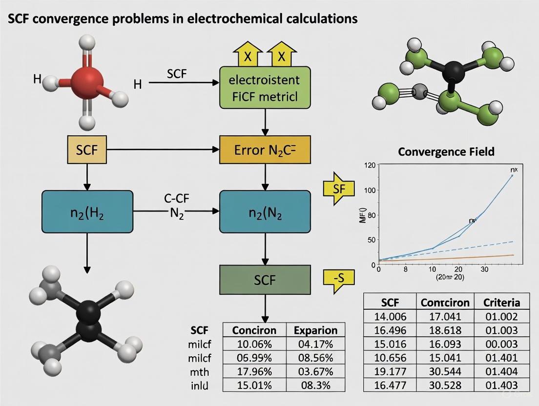
Overcoming SCF Convergence Challenges in Electrochemical Calculations: A Guide for Computational Researchers
Self-Consistent Field (SCF) convergence presents a significant hurdle in computational electrochemistry, where systems often feature small HOMO-LUMO gaps, open-shell configurations, and complex solute-electrode interactions.
Overcoming SCF Convergence Challenges in Electrochemical Calculations: A Guide for Computational Researchers
Abstract
Self-Consistent Field (SCF) convergence presents a significant hurdle in computational electrochemistry, where systems often feature small HOMO-LUMO gaps, open-shell configurations, and complex solute-electrode interactions. This article provides a comprehensive guide for researchers and scientists, exploring the foundational causes of convergence failure in electrochemical systems, detailing specialized methodological approaches like Grand Canonical DFT and advanced SCF algorithms, offering practical troubleshooting and optimization strategies from multiple quantum chemistry packages, and discussing validation techniques to ensure physically meaningful results. By synthesizing current methodologies and best practices, this work aims to enhance the reliability and efficiency of quantum chemical simulations in electrocatalysis and biomedical applications.
Why Electrochemical Systems Challenge SCF Solvers: Root Causes and Electronic Structure Complexities
The Unique Convergence Landscape of Electrochemical Systems
Frequently Asked Questions (FAQs)
Q1: What does "SCF convergence" mean in the context of electrochemical calculations? Self-Consistent Field (SCF) convergence is the process of iteratively solving the electronic structure equations until the energy and electron density of the system no longer change significantly between cycles. In electrochemical systems, this process is complicated by the presence of conductive electrodes, liquid electrolytes, and the application of an electrical potential, making convergence more difficult to achieve than in standard chemical systems. [1] [2]
Q2: My calculation stops with an "SCF convergence failure" error. What are the first steps I should take? Initial troubleshooting steps should follow a logical isolation process [3] [4]:
- Simplify the System: Test your setup on a smaller, known system to verify your methodology.
- Check Initial Guess: Ensure you are starting from a sensible initial electron density and wavefunction. A poor initial guess is a common culprit.
- Increase SCF Iterations: Temporarily increase the maximum number of SCF steps to rule out an overly strict limit.
- Verify Electrode Model: Confirm that your model of the electrochemical interface (e.g., slab thickness, vacuum/water layer size) is physically sound and properly constructed to avoid spurious interactions. [2]
Q3: How does the application of an electrode potential affect SCF convergence? The grand canonical (constant potential) approach, essential for modeling working electrochemical conditions, directly controls the electron chemical potential of the system. This explicit potential control alters the electronic structure landscape and can introduce states that are challenging for standard SCF algorithms to resolve, often requiring specialized techniques like Fermi smearing or density mixing to ensure stable convergence. [1]
Q4: Why are electrochemical interfaces particularly challenging for SCF algorithms? Electrochemical interfaces represent a complex convergence landscape due to several factors [2]:
- Physical Complexity: They involve a junction between a solid conductor (electrode) and a liquid ionic solution (electrolyte), each with vastly different dielectric properties.
- Multiple Components: The system contains a diverse mix of atoms (metals, oxygen, hydrogen, various ions) with different electronegativities and bonding characteristics. [5]
- Dynamic Nature: The interface is not static; atoms, particularly protons in water, are in constant motion, leading to a fluctuating electronic environment. [2]
Troubleshooting Guide: A Step-by-Step Walkthrough
Follow this structured guide to diagnose and resolve SCF convergence problems in your electrochemical simulations.
Step 1: Dummy Cell Test (Methodology Verification) Before introducing the full complexity of an electrochemical cell, verify your computational setup and methodology.
- Action: Perform a calculation on a simple, well-understood redox couple or a bulk piece of your electrode material using the same computational settings (functional, basis set, pseudopotentials).
- Expected Outcome: The calculation should converge smoothly.
- Interpretation: If this fails, the problem lies with your core computational parameters, not the interface model. If it passes, proceed to Step 2. [3]
Step 2: Isolate the Problem Component Reintroduce complexity gradually to identify the problematic component.
- Action 1: Test the Electrode in Vacuum. Run an SCF calculation on your electrode slab without the electrolyte. If it converges, the issue is likely related to the electrolyte or the interface.
- Action 2: Test the Electrolyte Separately. Run a molecular dynamics simulation of your electrolyte solution using a classical force field to ensure its structure is equilibrated before introducing it to the DFT calculation. [2]
- Interpretation: This process helps you determine whether to focus troubleshooting efforts on the electrode, the electrolyte, or their interaction.
Step 3: System-Specific Checks Based on the outcome of Step 2, perform targeted checks.
If the problem is with the electrode or initial setup:
- Check for Metallic Systems: For metallic electrodes like Pt(111) or Au(111), standard SCF methods can fail. Use techniques like Fermi smearing with an electronic temperature (e.g., 300 K) and Broyden density mixing to help convergence. [2]
- Verify Slab Stoichiometry: Ensure your electrode slab is stoichiometric to avoid introducing excess charge or holes that can prevent convergence. [2]
- Improve Initial Guess: Use the electron density from a related, converged calculation as a starting point for your target system.
If the problem is with the interface or electrolyte:
- Ensure Proper Solvation: Confirm that the water density in the bulk-like region of your model is correct (~1 g/cm³). [2]
- Check for Ionic Conductivity: In a real electrochemical cell, the electrolyte must conduct ions to complete the circuit. While this is explicitly modeled in simulations, a poorly constructed interface model can mimic a blocked circuit, leading to instability. Ensure no artificial barriers (like an excessively large vacuum gap) are preventing ion stabilization in the model. [3] [6]
Step 4: Advanced SCF Tuning If the above steps do not resolve the issue, advanced tuning of the SCF procedure is required. The table below summarizes key parameters and their typical values for challenging electrochemical systems.
Table 1: SCF Algorithm Parameters for Electrochemical Systems
| Parameter | Standard Value | Recommended for Challenging Systems | Function |
|---|---|---|---|
| SCF Convergence Threshold | ( 1 \times 10^{-6} ) a.u. | ( 1 \times 10^{-5} ) a.u. (loosen initially) | Target accuracy for the wavefunction optimization. |
| Fermi Smearing | N/A | 300 K (for metals) | Smears electronic occupancy around Fermi level, aiding metallic convergence. |
| Mixing Method | Simple/DIIS | Broyden / Pulay | Improves the update of the electron density between cycles. |
| Mixing Fraction | 0.05-0.2 | 0.05-0.1 | The fraction of new density mixed into the old. Too high can cause oscillation. |
| Algorithm (Non-Metallic) | DIIS | Orbital Transformation (OT) | OT can be more robust and faster for insulating systems. |
| Algorithm (Metallic) | DIIS | Second-Generation Car-Parrinello (SGCP) | SGCP is efficient for metals and large systems. [2] |
Experimental Protocols
Protocol: Evaluating the Effect of Potential on Electrochemical Reactions Using a Grand Canonical Method
This protocol outlines the steps for performing fixed-potential calculations, which are central to modeling electrochemical systems and are prone to SCF convergence issues. [1]
1. Software and Prerequisites
- Software: Install a DFT package capable of grand canonical calculations, such as CP2K/QUICKSTEP. [2]
- Knowledge: Familiarity with basic DFT concepts and the software's input file structure is assumed.
2. Preparing the Electrochemical Interface Model
- Slab Creation: Cleave the bulk crystal of your electrode material along the desired facet (e.g., Pt(111), SnO2(110)). Create a symmetric slab to avoid a net dipole moment perpendicular to the surface. [2]
- Solvation: Use a tool like PACKMOL to fill a simulation box with water molecules at a density of 1 g/cm³. Equilibrate this water box using classical molecular dynamics with a force field like SPC/E. [2]
- Interface Construction: Merge the equilibrated slab and water box to create the initial interface structure. Saturate under-coordinated surface atoms with water molecules where possible.
- Equilibration: Perform a short (e.g., 20-30 ps) ab initio molecular dynamics (AIMD) simulation of the full interface to equilibrate the structure at the target temperature (e.g., 330 K). Use the final snapshot of this simulation as the starting point for your fixed-potential calculations. [2]
3. Configuring the Fixed-Potential Calculation
- Input File Setup: In your DFT input file, activate the settings for grand canonical DFT calculations. This typically involves specifying the electron chemical potential (the potential) and the charge of the system.
- SCF Parameters: Set the SCF parameters as detailed in Table 1. For metallic electrodes, ensure Fermi smearing and a robust mixing algorithm like Broyden are enabled.
- Convergence Aids: It is often beneficial to first run a calculation with a looser SCF convergence criterion and use the resulting electron density as the initial guess for the production run with tighter criteria.
4. Execution and Analysis
- Run the Calculation: Submit the job and monitor the SCF convergence in the output file.
- Analyze Output: Upon successful convergence, analyze the resulting charge distribution, density of states, and free energy of the system at the applied potential to gain insight into the electrochemical reaction. [1]
The workflow for this protocol is summarized in the diagram below.
The Scientist's Toolkit: Research Reagent Solutions
The following table lists key computational "reagents" and their functions in setting up and troubleshooting electrochemical calculations.
Table 2: Essential Computational Tools for Electrochemical Interface Modeling
| Item / Software | Function / Purpose | Example in Use |
|---|---|---|
| CP2K | A DFT package specializing in atomistic simulations of condensed matter systems, particularly efficient for molecular dynamics and systems with large unit cells. | Used for running AIMD simulations of Pt(111)-water interfaces with Gaussian and plane-wave basis sets. [2] |
| LAMMPS | A classical and (with plugins) quantum molecular dynamics simulator. | Used for running MLMD (Machine Learning Molecular Dynamics) simulations with potentials from DeePMD-kit. [2] |
| DeePMD-kit | A package for building and running machine learning potentials (MLPs) trained on DFT data. | Used to create MLPs that extend simulation timescales to nanoseconds while maintaining AIMD accuracy. [2] |
| DP-GEN / ai2-kit | Concurrent learning packages for automatically generating training datasets for MLPs. | Used in an active learning workflow to explore the configuration space of an interface and build robust MLPs. [2] |
| PACKMOL | A tool for setting up initial configurations of molecular dynamics simulations by packing molecules in defined regions. | Used to fill a simulation box with water molecules to create an electrolyte solution for the interface model. [2] |
| SPC/E Water Model | A classical, rigid water model used for force-field-based equilibration of the electrolyte. | Used to pre-equilibrate the water box before merging it with the DFT-level electrode slab. [2] |
| Goedecker-Teter-Hutter (GTH) Pseudopotentials | Pseudopotentials that describe the core electrons, freeing up computational resources for valence electrons. | Standard in CP2K simulations to describe core-electron interactions for elements like O, H, Zn, Mn, etc. [2] |
| Perdew-Burke-Ernzerhof (PBE) Functional | A popular generalized gradient approximation (GGA) exchange-correlation functional in DFT. | Commonly used to describe electron interactions in electrochemical interface studies, though it has known limitations for van der Waals forces and band gaps. [2] |
Impact of Small HOMO-LUMO Gaps and Metallic Character on SCF Stability
FAQs on SCF Convergence in Electrochemical Systems
1. Why do my electrochemical interface calculations, particularly for metals or small-gap semiconductors, frequently fail to converge?
Systems with small or zero HOMO-LUMO gaps, such as metals or certain semiconductor electrodes, present a fundamental challenge for the Self-Consistent Field (SCF) procedure. The core issue is that the energetic ordering of molecular orbitals can switch during the iterative SCF optimization. This leads to discontinuities in the optimization process, resulting in very slow convergence or outright failure [7]. In metallic systems, the presence of many near-degenerate electronic levels around the Fermi level exacerbates this problem [8].
2. What are the primary computational strategies to stabilize SCF convergence for such challenging systems?
Two main strategies, often used in conjunction, are employed:
- Fractional Orbital Occupations: This technique smears the electron occupation over several orbitals near the Fermi level, mimicking a finite electronic temperature. This prevents sharp, discontinuous changes in the density matrix when orbital energies cross, thereby stabilizing the SCF cycle [7] [2].
- Advanced SCF Accelerators and Parameters: Using more robust SCF convergence algorithms and carefully tuning their parameters can significantly improve stability. This includes methods like DIIS with a larger number of expansion vectors and lower mixing parameters, or alternative algorithms like MESA, LISTi, EDIIS, and the Augmented Roothaan-Hall (ARH) method [8].
3. How does the choice of basis set and planewave cutoff in CP2K/QUICKSTEP calculations affect SCF stability for metallic interfaces?
In the CP2K code, which uses a mixed Gaussian and plane-wave (GPW) basis set, convergence must be approached for both the Gaussian basis set and the auxiliary plane-wave basis concurrently. An insufficiently high plane-wave cutoff (CUTOFF in the &MGRID section) for the electron density can lead to numerical inaccuracies that destabilize the SCF process, especially for metals with delocalized electrons. It is crucial to increase the cutoff toward the complete basis set limit to ensure a stable and accurate calculation [9].
Troubleshooting Guide: Resolving SCF Instabilities
Step 1: Initial System Checks
Before adjusting advanced parameters, rule out simple issues.
- Verify Geometry: Ensure your electrochemical interface model has realistic bond lengths and angles. A high-energy, non-physical geometry is a common root cause of convergence problems [8].
- Confirm Spin Multiplicity: For systems containing transition metals (e.g., Pt, CoO), ensure you are using the correct spin multiplicity and an unrestricted spin formalism if needed [8].
- Reuse Converged Potentials: In a geometry optimization, use a moderately converged electronic structure from a previous step as the initial guess for the next step [8].
Step 2: Algorithm Selection and Parameter Tuning
If basic checks pass, proceed to adjust SCF controls. The following table summarizes key parameters for the DIIS algorithm, which can be adjusted for a "slow but steady" convergence approach [8].
| Parameter | Standard Default | Recommended Value for Problematic Systems | Explanation |
|---|---|---|---|
| Mixing | 0.2 | 0.015 | Fraction of new Fock matrix used. Lower values increase stability. |
| Mixing1 | 0.2 | 0.09 | Mixing parameter for the very first SCF cycle. |
| N (DIIS Vectors) | 10 | 25 | Number of previous steps used for extrapolation. More vectors increase stability. |
| Cyc (Start Cycle) | 5 | 30 | Number of initial SCF cycles before DIIS acceleration starts. |
Example input for a difficult system in a typical DFT code:
Step 3: Employing Electron Smearing and Fractional Occupations
For systems with a vanishing HOMO-LUMO gap (metals, narrow-gap semiconductors), enforcing fractional orbital occupations is often the most effective solution. The table below outlines the key parameters for the pseudo-Fractional Occupation Number (pFON) method [7].
| Parameter | Description | Recommended Setting |
|---|---|---|
| OCCUPATIONS | Activates fractional occupations. | 2 (for pFON) |
| FONTSTART | Initial electronic temperature (K). | 300 K (room temperature) or higher for difficult cases. |
| FONTEND | Final electronic temperature (K). | 300 K or as low as possible. |
| FON_NORB | Number of orbitals above/below Fermi level for smearing. | Number of valence orbitals (e.g., 10). |
| FONETHRESH | DIIS error threshold to freeze occupations. | 5 (freeze at 10⁻⁵) or one step above your SCF convergence criterion. |
Example input for a Pt system using pFON in Q-Chem [7]:
Note: Electron smearing alters the total energy. The smearing parameter (electronic temperature) should be kept as low as possible, and multiple restarts with successively smaller values can be used to approach the zero-temperature limit [8].
Step 4: Utilizing Advanced SCF Accelerators
If DIIS and smearing are insufficient, consider switching the SCF convergence accelerator. The Augmented Roothaan-Hall (ARH) method, for instance, directly minimizes the total energy and can be a viable, though computationally more expensive, alternative for the most difficult cases [8].
Experimental Protocols for Electrochemical Interface Modeling
The following workflow, based on the methodology used to create the ElectroFace dataset, details the steps for generating a stable and physically meaningful model of an electrochemical interface for AIMD or MLMD simulations [2].
Key steps in the workflow:
- Slab Preparation: Generate a symmetric, stoichiometric slab from the bulk crystal to avoid spurious dipole interactions and excess charge [2].
- Water Phase Equilibration: Create and classically equilibrate a box of water molecules to ensure a realistic liquid structure before introducing the interface [2].
- Density Adjustment: Iteratively run short AIMD simulations and adjust the number of water molecules until the density in the bulk-like region of the liquid phase is correct (1.0 g/cm³ within a 5% error margin). This ensures the interface model is physically realistic [2].
- Production Run: Use the final, validated structure from step 3 to launch extended AIMD or machine-learning accelerated MD (MLMD) simulations [2].
The Scientist's Toolkit: Research Reagent Solutions
The table below lists essential computational "reagents" and their functions for managing SCF convergence in electrochemical simulations.
| Item / Method | Function / Purpose |
|---|---|
| pFON (pseudo-Fractional Occupation Numbers) | Smears electron occupation over near-degenerate orbitals to stabilize SCF in metallic/small-gap systems [7]. |
| Fermi Smearing | Alternative to pFON; uses a Fermi-Dirac distribution for orbital occupation at a finite electronic temperature (e.g., 300 K) [2]. |
| DIIS (Direct Inversion in Iterative Subspace) | Standard SCF convergence accelerator; parameters (N, Mixing) can be tuned for stability [8]. |
| ARH (Augmented Roothaan-Hall) | Alternative, robust SCF minimizer used when DIIS fails [8]. |
| Machine Learning Potentials (DeePMD-kit) | Enables nanosecond-scale MD simulations at near-DFT accuracy after training on AIMD data, bypassing direct SCF convergence in long runs [2]. |
| Grimme D3 Dispersion Correction | Accounts for van der Waals interactions, critical for accurate description of adsorption and interface structure [2]. |
| GTH Pseudopotentials | Represents core electrons, reducing computational cost while maintaining accuracy for valence electrons [2]. |
| SPC/E Water Force Field | A classical model used for the efficient pre-equilibration of the water phase before QM/MM or pure AIMD simulations [2]. |
SCF Convergence Decision Workflow
When faced with an SCF convergence problem, follow this logical pathway to identify and apply the appropriate solution.
Challenges of Open-Shell Configurations in Transition Metal Complexes and Radicals
Troubleshooting Guide: Resolving SCF Convergence Failures
Q: My SCF calculation for an open-shell transition metal complex fails to converge. What are the primary causes and immediate steps I should take?
A: Self-Consistent Field (SCF) convergence failures are common when calculating open-shell transition metal systems due to their complex electronic structures. The main physical reasons include small HOMO-LUMO gaps leading to oscillating orbital occupations, open-shell electronic configurations with localized d-orbitals, and issues with the initial orbital guess [8] [10] [11]. Systems with magnetic anisotropy or near-degenerate states are particularly problematic [12] [11].
Immediate troubleshooting steps:
- Verify Molecular Geometry: Ensure bond lengths and angles are chemically reasonable. Check coordinate units and for unrealistic close contacts [8] [11].
- Confirm Spin Multiplicity: Use the correct spin-unrestricted formalism and manually set the total spin if necessary [8].
- Use a Better Initial Guess: Converge a simpler method (e.g., BP86/def2-SVP) and read orbitals for a restart, or try
PAtom,Hueckel, orHCoreguesses [10]. - Increase SCF Iterations: For calculations nearly converged, increase the maximum iteration count (e.g.,
%scf MaxIter 500 end) [10].
Q: Which SCF convergence algorithms and parameters are most effective for difficult open-shell cases?
A: Standard DIIS algorithms often struggle. For difficult cases in ORCA, employ dedicated convergence keywords and parameter adjustments.
Table: SCF Convergence Algorithms and Settings for Open-Shell Systems
| Method/Setting | Description | Typical Use Case | ORCA Input Example |
|---|---|---|---|
| SlowConv/VerySlowConv | Increases damping to stabilize large initial density fluctuations [10]. | General purpose for oscillating SCF. | ! SlowConv |
| KDIIS with SOSCF | Alternative algorithm, often faster than DIIS [10]. | When standard DIIS is slow or fails. | ! KDIIS SOSCF |
| TRAH (Trust Radius Augmented Hessian) | Robust second-order converger, automatically activates in ORCA 5+ if DIIS struggles [10] [13]. | Pathological cases; guarantees a local minimum [13]. | (Active by default) |
| Level Shifting | Artificially raises virtual orbital energies to prevent oscillation [8] [10]. | Small HOMO-LUMO gaps. | %scf Shift Shift 0.1 end |
| DIIS Parameter Adjustment | Using more expansion vectors (DIISMaxEq) increases stability [10]. |
Severe convergence problems (e.g., metal clusters). | %scf DIISMaxEq 25 end |
| Electron Smearing | Uses fractional occupations to help converge metallic systems or those with near-degenerate states [8]. | Very small or zero HOMO-LUMO gap. | %scf Smear 0.01 end |
For pathological cases (e.g., metal clusters), a combination of settings is often required [10]:
Q: How do I select appropriate convergence tolerances for production calculations on transition metal complexes?
A: Tighter-than-default tolerances are often necessary. ORCA provides predefined convergence keywords. The TightSCF criterion is recommended for transition metal complexes [13].
Table: SCF Convergence Tolerances in ORCA (Selected) [13]
| Criterion | LooseSCF | MediumSCF | StrongSCF | TightSCF | Description |
|---|---|---|---|---|---|
| TolE | 1e-5 | 1e-6 | 3e-7 | 1e-8 | Energy change between cycles. |
| TolMaxP | 1e-3 | 1e-5 | 3e-6 | 1e-7 | Maximum density change. |
| TolRMSP | 1e-4 | 1e-6 | 1e-7 | 5e-9 | RMS density change. |
| TolErr | 5e-4 | 1e-5 | 3e-6 | 5e-7 | DIIS error convergence. |
FAQ: Addressing Common Computational Challenges
Q: How significant are relativistic and dispersion effects on the conformational energies of open-shell 3d metal complexes?
A: The influence depends on the metal and ligand environment. For first-row (3d) transition metals, scalar relativistic effects on conformational energies are generally negligible [12]. In contrast, intramolecular dispersion interactions (e.g., from Grimme's D3 correction with BJ damping) can be crucial, especially for complexes with bulky substituents in close proximity [12]. Always account for dispersion in such systems.
Q: What fast computational methods provide reliable conformational energies for open-shell transition metal complexes?
A: Performance varies significantly across methods. A study on the 16OSTM10 database shows that while cheap methods are available, they should be used cautiously [12].
Table: Performance of Computational Methods for OSTM Conformational Energies [12]
| Method Class | Examples | Average Pearson Correlation (ρ) with Reference DFT | Recommendation |
|---|---|---|---|
| Conventional DFT | PBE-D3(BJ), PBE0-D3(BJ), ωB97X-V | 0.91 | Reliable reference methods. |
| Composite DFT | PBEh-3c, B97-3c | 0.93 | Good balance of speed and accuracy. |
| Semiempirical (GFNn) | GFN1-xTB, GFN2-xTB | 0.75 | Moderate performance; use with caution. |
| Force Field | GFN-FF | 0.62 | Poor performance; not recommended. |
| Semiempirical (Traditional) | PM6, PM7 | 0.53 | Poor performance; avoid. |
Q: My system has a very small or zero HOMO-LUMO gap. What specific techniques can help achieve convergence?
A: Small gaps cause "charge sloshing" and orbital occupation flipping [11]. Solutions include:
- Electron Smearing: Apply a small finite electron temperature (
%scf Smear 0.001 end), gradually reducing it in subsequent restarts [8]. - Level Shifting: This stabilizes the SCF procedure [8] [10].
- Converge a Closed-Shell State: If possible, converge a 1- or 2-electron oxidized/reduced (closed-shell) state and use its orbitals as a guess for the target open-shell system [10].
- Use a Sufficiently Accurate Grid: Numerical noise from an insufficient integration grid can prevent convergence [10] [11].
Experimental Protocols & Workflows
Protocol 1: Systematic Conformational Search for Flexible Open-Shell Complexes This methodology is adapted from the creation of the 16OSTM10 database [12].
- Initial Structure Selection: Retrieve structures from crystallographic databases (e.g., CSD). Select complexes with a first-row transition metal, an open-shell ground state, and at least 5 rotatable bonds.
- Ground State Optimization: Optimize the initial structure at the
PBE-D3(BJ)/def2-SVPlevel, testing relevant spin multiplicities. Re-evaluate energy at a higher level (e.g.,PBE0-D3(BJ)/def2-TZVP) to confirm the ground state. - Multireference Diagnostics: Perform
DLPNO-CCSD(T)/cc-pVDZcalculations to obtain T1/T2 diagnostics. Exclude compounds with significant multireference character (T1 > 0.025 or T2 > 0.15) if using single-reference methods [12]. - Conformer Generation: Use an automated algorithm to generate 30-35 spatially diverse conformers.
- Pre-optimization: Pre-optimize all conformers using a fast, low-cost method (e.g.,
PBE/λ1in Priroda) [12]. - Final Optimization and Energy Benchmarking: Optimize unique conformers at the
PBE-D3(BJ)/def2-SVPlevel. Calculate final single-point energies for all conformers using a robust reference method (e.g.,PBE0-D3(BJ)/def2-TZVPorωB97X-V/def2-TZVP) to build the conformational energy profile.
Workflow for Conformational Energy Benchmarking
Protocol 2: Robust SCF Convergence Protocol for Problematic Systems This protocol combines recommendations from ORCA and ADF documentation [8] [10].
- Initial Checks: Verify geometry and spin state.
- Standard SCF Procedure: Run with default settings. If it converges, proceed.
- Enable Robust Converger: If slow or oscillating, use
! SlowConvor allowTRAHto activate automatically [10] [13]. - Advanced DIIS Tuning: For persistent failure, increase DIIS memory (
DIISMaxEq) and reduce Fock matrix rebuild frequency (directresetfreq) [10]. - Improved Initial Guess: Converge a simpler method or different charge/spin state and restart with
! MORead[10]. - Last Resort - Smearing/Shifting: For systems with tiny HOMO-LUMO gaps, apply minimal electron smearing or level shifting [8].
Troubleshooting Protocol for SCF Convergence
The Scientist's Toolkit: Essential Research Reagents & Materials
Table: Key Computational Tools for Open-Shell Transition Metal Research
| Item / Resource | Function / Description | Application Note |
|---|---|---|
| 16OSTM10 Database | A benchmark database of 10 conformations for each of 16 open-shell TM complexes [12]. | Used for validation and training of fast methods (SE, FF, ML). |
| Composite DFT Methods (B97-3c, PBEh-3c) | Low-cost DFT methods with minimized basis sets and built-in corrections [12]. | Good speed/accuracy for conformational energies (ρ ≈ 0.93) [12]. |
| GFNn-xTB Methods | Semiempirical methods with generally good performance for geometries and energies [12]. | Use with caution for OSTM conformational energies (average ρ = 0.75) [12]. |
| D3(BJ) Dispersion Correction | Adds empirical dispersion interactions to DFT [12]. | Crucial for complexes with bulky ligands [12]. |
| DLPNO-CCSD(T) | High-level wavefunction method for accurate energies and diagnostics [12]. | Used for T1/T2 diagnostics to exclude multireference systems [12]. |
| ROCIS Method | Restricted Open-Shell CI Singles method for spectroscopy [14]. | Calculates transition metal L-edge X-ray absorption spectra including spin-orbit coupling [14]. |
| TRAH SCF Algorithm | Trust Radius Augmented Hessian SCF converger [10] [13]. | Robust second-order method for difficult cases; default in ORCA 5+ [10]. |
The Role of Diffuse Basis Sets and Fractional Electrons in Constant-Potential Calculations
Frequently Asked Questions (FAQs)
FAQ 1: Why are my electrochemical calculations failing to converge, and how are diffuse basis sets involved?
SCF convergence problems are frequently encountered in systems with very small HOMO-LUMO gaps, which are common in electrochemical environments and systems with dissociating bonds [8]. Diffuse basis sets, while essential for accuracy in describing non-covalent interactions and anions, significantly reduce the sparsity of the one-particle density matrix [15]. This "curse of sparsity" leads to a late onset of the low-scaling regime and larger cutoff errors, making convergence more difficult and computationally expensive [15].
FAQ 2: What is the relationship between fractional electrons and constant-potential calculations?
In the context of simulating electrochemical reactions, a Grand Canonical approach within density functional theory can be used where fractional numbers of electrons represent an open system in contact with an electrode at a given electrochemical potential [16]. This approach explicitly includes the electrochemical potential, allowing for the modeling of systems where electron exchange with a reservoir is possible.
FAQ 3: When should I use diffuse functions in my basis set for electrochemical calculations?
Diffuse functions are essential for obtaining accurate interaction energies, particularly for non-covalent interactions and charged species common in electrochemical environments [15]. However, they come with a significant computational cost and can hinder SCF convergence. They should be used when studying processes where electron density is more dispersed, such as in anions, excited states, or weak interactions, but may be avoided in initial calculations on challenging systems to establish convergence first [15].
FAQ 4: What practical SCF convergence techniques can I implement for difficult systems?
For problematic SCF convergence, several techniques can be employed:
- Change to different SCF convergence acceleration methods like MESA, LISTi, or EDIIS [8]
- Adjust DIIS parameters: increase the number of expansion vectors (N=25), increase initial cycles before DIIS starts (Cyc=30), and reduce mixing parameters (Mixing=0.015) for more stable convergence [8]
- Utilize electron smearing to simulate a finite electron temperature using fractional occupation numbers, which helps overcome convergence issues in systems with many near-degenerate levels [8]
Troubleshooting Guides
Guide 1: Addressing SCF Convergence Failures in Electrochemical Calculations
Symptoms: SCF cycles oscillate without converging, calculations terminate due to maximum cycle limits, or energies fluctuate wildly.
Diagnosis and Solutions:
Verify System Physicality
Validate Electronic Structure Description
Implement Advanced SCF Accelerators
- Switch from default DIIS to alternative methods like ARH (Augmented Roothaan-Hall) for difficult systems [8]
- Use the following parameter set as a starting point for problematic cases:
Apply Electron Smearing or Level Shifting
- Implement electron smearing with fractional occupation numbers to distribute electrons over near-degenerate levels [8]
- Use level shifting to artificially raise virtual orbital energies (note: this affects properties involving virtual levels) [8]
- Keep smearing values as low as possible and use successive restarts with reduced values [8]
Guide 2: Managing Basis Set Selection Trade-offs
Symptoms: Accurate results require diffuse functions but make calculations computationally prohibitive or unstable.
Diagnosis and Solutions:
Understand the Accuracy-Sparsity Trade-off
Table 1: Basis Set Performance for Non-Covalent Interactions (NCI) with ωB97X-V Functional
Basis Set NCI RMSD (M+B) (kJ/mol) Time (s) for DNA Fragment def2-SVP 31.51 151 def2-TZVP 8.20 481 def2-TZVPPD 2.45 1440 aug-cc-pVDZ 4.83 975 aug-cc-pVTZ 2.50 2706 aug-cc-pV6Z 2.41 57954 Data adapted from [15]. RMSD values reference aug-cc-pV6Z. M+B indicates combined method and basis set error.
Implement Strategic Basis Set Selection
- Use def2-TZVPPD or aug-cc-pVTZ as minimum for accurate NCI results [15]
- For initial scans, use smaller basis sets without diffuse functions, then refine with diffuse-augmented basis sets
- Consider the CABS (complementary auxiliary basis set) singles correction with compact, low l-quantum-number basis sets as an alternative [15]
Employ Mixed Basis Set Approaches
- Use different basis sets for different atoms via the
genkeyword [17] - Apply more complete basis sets to reactive centers and smaller basis sets to spectator atoms
- Example implementation for a platinum complex:
- Use different basis sets for different atoms via the
Guide 3: Implementing Constant-Potential Methods with Fractional Electrons
Symptoms: Difficulty maintaining constant potential in electrochemical simulations or representing open systems.
Diagnosis and Solutions:
Establish Grand Canonical DFT Framework
- Implement fractional electron counts to represent open systems in contact with electrodes [16]
- Develop SCF procedures that accommodate fractional electron numbers with minimal additional computational effort [16]
- Combine with implicit solvent models to represent electrochemical environments [16] [18]
Address Computational Challenges
- Utilize moderately converged electronic structures from previous calculations as initial guesses [8]
- Implement robust convergence criteria that account for fractional occupation effects
- Employ restart capabilities to build upon partially converged wavefunctions
Experimental Protocols and Methodologies
Protocol 1: Systematic Approach for Difficult SCF Convergence
Initial Setup and Validation
Gradual Refinement Procedure
Final Calculation with Diffuse Functions
- Employ previously converged density as initial guess
- Use aggressive SCF convergence criteria (8-10 cycles) [18]
- Monitor SCF behavior for oscillations and adjust mixing parameters if needed
Protocol 2: Basis Set Selection Strategy for Electrochemical Systems
Accuracy Requirement Assessment
- Determine whether non-covalent interactions, anion characterization, or charge transfer processes are central to the study
- Reference Table 1 to select appropriate basis set based on target accuracy and computational resources [15]
Progressive Basis Set Approach
- Conduct geometry optimizations with moderate basis sets (def2-SVP, def2-TZVP)
- Perform single-point energy calculations with diffuse-augmented basis sets (def2-TZVPPD, aug-cc-pVTZ)
- For highest accuracy, utilize progressively larger basis sets (cc-pVQZ, cc-pV5Z) with diffuse functions [15]
The Scientist's Toolkit
Table 2: Essential Computational Resources for Electrochemical Calculations
| Resource/Technique | Function | Application Context |
|---|---|---|
| Diffuse-Augmented Basis Sets | Accurately describe non-covalent interactions, anions, and dispersed electron densities | Essential for interaction energies, charged species, excited states [15] |
| Electron Smearing | Enable convergence via fractional occupation of near-degenerate orbitals | Metallic systems, small-gap systems, transition states [8] |
| Effective Core Potentials (ECPs) | Reduce computational cost by replacing core electrons with pseudopotentials | Systems with heavy elements (transition metals, lanthanides) [17] |
| Implicit Solvent Models | Represent solvent effects without explicit solvent molecules | Electrochemical environments, solution-phase systems [18] |
| SCF Acceleration Algorithms (DIIS, DIIS-GDM, ARH) | Improve and stabilize SCF convergence | Problematic systems with small HOMO-LUMO gaps or open-shell configurations [8] [18] |
| Mixed Basis Set Approaches | Apply different basis sets to different atoms for efficiency balance | Large systems where accuracy is only needed at reactive centers [17] |
Workflow Visualization
Frequently Asked Questions
1. Why does my geometry optimization fail to converge or my molecule "explode"?
Geometry optimization failures can often be traced back to the initial structure. An implausible starting geometry—such as atoms placed too close together, or a mix-up between coordinate units (Angstroms vs. Bohr)—can cause the optimization to fail catastrophically [19]. Furthermore, for heavy elements, ensure you are using an appropriate basis set that includes necessary functions or an effective core potential (ECP) to properly describe the core electrons [19]. In rare cases, the optimizer's internal coordinate system may be unsuitable for your molecule; switching to a Cartesian coordinate system (using the !COpt keyword in ORCA) can resolve this [19].
2. What does an "imaginary vibrational mode" mean after a frequency calculation on my optimized structure?
Imaginary frequencies (reported as negative wavenumbers, e.g., -70 cm⁻¹) indicate that the optimized geometry is not a true minimum on the potential energy surface but a saddle point [19].
- Small imaginary modes (below ~100 cm⁻¹) are often caused by numerical noise. This can be addressed by increasing the integration grid size (e.g., moving from
!DefGrid2to!DefGrid3) or using the!TightOptkeyword for a more precise geometry optimization [19]. - Larger imaginary modes typically mean the optimization converged to a transition state instead of a minimum. This often happens when the starting geometry possesses high symmetry. The solution is to distort the starting geometry away from this symmetric structure [19].
3. My SCF calculation won't converge. What are the first things I should check?
Before adjusting advanced SCF settings, always verify the basics [19] [10]:
- Coordinates: Are the atom positions reasonable? Visualize them.
- Charge and Multiplicity: Are they correct for your system?
- Basis Set: Are you using a diffuse basis set (e.g.,
aug-cc-pVTZ)? These can cause linear dependency issues, making convergence difficult. Consider a less diffuse alternative [19]. - System Stability: Are you calculating an anion in the gas phase? It may be unstable without a solvation model (like CPCM) to stabilize it [19].
4. I see a "Not enough memory" error. How do I control memory in ORCA?
Memory in ORCA is controlled per core using the %maxcore keyword. The value is specified in MB. The total memory used is maxcore * number of cores [19].
- Example:
%maxcore 3000withnprocs 6uses 6 * 3000 = 18,000 MB (18 GB) total [19]. - Best Practice: Do not request more than 75% of the physical memory available on a node, as ORCA can occasionally use more than the
maxcoresetting [19].
5. What should I do if my geometry optimization stops because the SCF did not converge?
In ORCA, by default, a geometry optimization will stop if the SCF fails to converge in a given cycle [10]. You can modify this behavior, but a better strategy is to address the root cause of the SCF failure. Use the guidelines in the SCF convergence section below to stabilize the calculation. For a single-point energy calculation, ORCA will not proceed to post-HF steps if the SCF is not fully converged [10].
Troubleshooting Guides
Diagnosing and Fixing SCF Convergence Problems
Self-Consistent Field (SCF) convergence is fundamental to most quantum chemistry calculations. Follow this logical workflow to diagnose and resolve issues.
Detailed Methodologies for Key SCF Protocols:
- Addressing Numerical Noise: If you suspect the integration grid (DFT) or COSX grid (RIJCOSX approximation) is causing noise, increase the grid size. In ORCA, use
!DefGrid3for a tighter grid than the defaultDefGrid2[19]. - Using Damping Algorithms: For systems with large initial energy fluctuations (common in open-shell transition metal complexes), use the
!SlowConvor!VerySlowConvkeywords. These automatically increase damping to help guide the SCF to convergence [10]. - Specialist SCF Algorithms:
- KDIIS with SOSCF: The
!KDIIS SOSCFcombination can offer faster convergence for some difficult cases. If the SOSCF algorithm itself fails, you can delay its start with a%scf SOSCFStart 0.00033 endblock [10]. - Tweaking DIIS: For pathological cases (e.g., metal clusters), increase the number of Fock matrices used in the DIIS extrapolation inside the SCF block:
%scf DIISMaxEq 15 end(default is 5). You can also force a full rebuild of the Fock matrix every iteration withdirectresetfreq 1to eliminate numerical noise, though this is computationally expensive [10].
- KDIIS with SOSCF: The
Resolving Geometry and Import Errors
Incorrect molecular geometry is a primary cause of calculation failures. This includes both user-created structures and those imported from databases or other software.
Common Geometry Pitfalls and Solutions:
| Pitfall | Description | Solution |
|---|---|---|
| Invalid Starting Geometry | Atoms placed impossibly close or with unrealistic bond lengths/angles [19]. | Always visualize your structure before calculation. Use chemical knowledge to create a plausible initial geometry. |
| Unit Confusion | Accidentally using Bohr coordinates when the software expects Angstroms, or vice-versa [19]. | Double-check the input requirements of your computational chemistry software and ensure your coordinate file is saved in the correct unit. |
| Linear Dependency (Basis Set) | Using very large, diffuse basis sets (e.g., aug-cc-pVQZ) on systems with many atoms, leading to numerical instability [19] [10]. |
Use a smaller or less diffuse basis set. The ma-def2 series can be a good alternative to aug-cc-pV sets for some applications [19]. |
| Heavy Element Misconfiguration | Missing effective core potentials (ECPs) or key basis functions for heavy atoms [19]. | Consult basis set repositories (e.g., EMSL) to ensure you have a consistent basis set and ECP for all elements. Use the ! PrintBasis keyword in ORCA to verify. |
Experimental Protocol: Generating a Robust Initial Guess
For systems that are notoriously difficult to converge (e.g., open-shell transition metal complexes or conjugated radical anions), a multi-step protocol is recommended [10]:
- Simplify the System: Perform a single-point energy calculation using a simpler, more robust method and basis set (e.g., BP86/def2-SVP).
- Converge the Simple Calculation: Ensure the SCF converges for this simpler case. You may need to use
!SlowConvor other keywords from the troubleshooting guide above. - Read the Orbitals: Use the converged orbitals from the simple calculation as the starting guess for your more advanced target calculation (e.g., DLPNO-CCSD(T)/def2-TZVPP). This is done in ORCA with the
! MOReadkeyword and a%moinp "simple_calc.gbw"block [10]. - Proceed with Target Calculation: The advanced calculation will now begin from a much better initial guess, significantly improving the chances of SCF convergence.
The Scientist's Toolkit
Essential Research Reagent Solutions for Computational Electrochemistry
| Item | Function in Research |
|---|---|
| Continuum Solvation Model (e.g., CPCM) | Mimics the electrochemical environment (e.g., a solvent) by embedding the molecule in a polarizable continuum, crucial for calculating realistic redox potentials and stabilizing anions [19]. |
| Diffuse Basis Sets (e.g., aug-cc-pVXZ) | Provides a more accurate description of electron-rich regions, such as those in anions or excited states, which are critical in electron transfer processes [19]. |
| Effective Core Potential (ECP) | Replaces the core electrons of heavy atoms with a potential, reducing computational cost and allowing the study of transition metal catalysts prevalent in electrochemical systems [19]. |
| Integration Grid (e.g., DefGrid1-3) | The numerical grid used to integrate the Exchange-Correlation functional in DFT. A finer grid (higher number) reduces numerical noise, which is essential for stable geometry optimizations and frequency calculations [19]. |
| SCF Convergence Accelerators (e.g., DIIS, SOSCF) | Algorithms that help the SCF procedure find a stable solution for the electron density, which is often challenging for the open-shell species common in electrochemistry [10]. |
Advanced SCF Algorithms and Constant-Potential Methods for Electrochemical Simulations
Theoretical Foundation and Key Concepts
What is Grand Canonical DFT (GCDFT) and how does it differ from standard DFT?
Answer: Grand Canonical Density Functional Theory (GCDFT) is an extension of traditional DFT that enables calculations at a constant electrochemical potential (μ), rather than with a fixed number of electrons. This approach is particularly crucial for modeling electrochemical systems where electron transfer occurs at electrode-electrolyte interfaces. In standard canonical ensemble DFT, the electron number (N) is fixed, and the total electronic energy (E) is minimized. In contrast, GCDFT minimizes the grand canonical free energy (Ω) defined as:
Ω = EDFT - μN - (1/β)Sel
where EDFT is the DFT electronic energy, μ is the chemical potential, N is the electron number, β is the inverse temperature, and Sel is the electronic entropy. This formulation allows the electron number to vary adaptively between self-consistent field (SCF) iterations, making it particularly suitable for simulating electrochemical processes under constant potential conditions [20] [21].
What are the primary applications of GCDFT in electrochemical research?
Answer: GCDFT has become an indispensable tool in computational electrochemistry with several key applications:
- Electrocatalyst Screening: High-throughput discovery of efficient catalysts for reactions such as hydrogen evolution, oxygen reduction, and CO₂ reduction
- Battery Material Design: Investigation of electrode-electrolyte interfaces in lithium-ion and beyond-lithium batteries
- Corrosion Studies: Modeling dissolution and passivation processes at metal surfaces under electrochemical potential control
- Interface Phenomena: Understanding potential-dependent solvent reorganization and ion adsorption at solid-liquid interfaces The unique capability to explicitly control electrode potential in first-principles calculations enables researchers to directly simulate experimental conditions and predict thermodynamic and kinetic parameters for electrochemical reactions [20] [21].
Implementation and Methodology
What is the computational workflow for implementing GCDFT?
Answer: Implementing GCDFT requires a self-consistent procedure that simultaneously optimizes the electron density and chemical potential. The following diagram illustrates the key computational workflow:
The implementation differs significantly from conventional DFT in its direct minimization of the grand canonical potential over density matrices with adaptive updating of electron number between SCF iterations. This approach stores the one-electron reduced density matrix (1RDM) as the central variational parameter, which is more practical in Gaussian-type orbital (GTO) bases than in plane-wave frameworks due to storage considerations [20].
What basis sets and solvation models are recommended for GCDFT calculations?
Answer: The choice of basis sets and solvation models critically impacts the accuracy and efficiency of GCDFT simulations:
Table: Essential Computational Components for GCDFT Implementation
| Component | Type/Options | Purpose in GCDFT | Key Considerations |
|---|---|---|---|
| Basis Sets | Gaussian-type orbitals (GTOs) | Discretize Hamiltonian and density matrices | Recently developed GTOs that extrapolate to basis set limit are recommended [20] |
| Solvation Models | Implicit linear dielectric + ionic response | Model solvent/electrolyte environment | Introduces <50% overhead vs. gas-phase; essential for interfacial electrochemistry [20] |
| XC Functionals | PBE, PBEsol, vdW-DF-C09 | Approximate exchange-correlation | PBEsol and vdW-DF-C09 show lower errors in oxide materials [22] |
| Grand Canonical Integrator | Variational minimization | Directly minimize Ω with adaptive electron number | More robust than Pulay mixing schemes; avoids multiple fixed-N calculations [20] |
For electrochemical applications, the integration of GCDFT with implicit solvation models that account for both linear dielectric response and ionic screening is particularly important. These solvation schemes introduce minimal computational overhead (less than 50% compared to gas-phase calculations) while enabling realistic modeling of solid-liquid interfaces [20].
Troubleshooting SCF Convergence Problems
Why does GCDFT present unique SCF convergence challenges?
Answer: GCDFT introduces additional complexity to SCF convergence due to the coupled optimization of electron density and chemical potential. Common issues include:
- Strong Density Oscillations: Large fluctuations in early iterations due to simultaneous updates of density matrix and electron number
- Charge Sling-shotting: Unphysical hopping between electron numbers when chemical potential is near degenerate energy levels
- Implicit Solvation Coupling: Additional self-consistency between electron density and solvent reaction field
- Small HOMO-LUMO Gaps: Metallic systems or those with near-degenerate states exacerbate convergence difficulties
These problems are particularly prevalent in transition metal complexes, open-shell systems, and materials with localized d- and f-electron configurations where multiple redox states compete energetically [8] [10] [20].
What specific strategies improve GCDFT SCF convergence?
Answer: Based on implementation experience across multiple codes, the following strategies have proven effective:
Table: SCF Convergence Accelerators for GCDFT Calculations
| Method | Mechanism | Best For | GCDFT Considerations |
|---|---|---|---|
| DIIS with Extended Subspace | Extrapolates Fock matrix using history | Most systems | Increase DIISMaxEq to 15-40 for difficult cases [10] |
| Damping | Mixes old and new Fock matrices | Initial oscillations | Apply 20-50% damping in first 5-10 cycles [8] [23] |
| Level Shifting | Artificially increases HOMO-LUMO gap | Small-gap systems | 0.1-0.3 Hartree shift; delays convergence but improves stability [8] [23] |
| Electron Smearing | Fractional occupancies via finite temperature | Metallic systems | Use multiple restarts with successively smaller smearing values [8] |
| Direct Minimization | Variational optimization of grand potential | Pathological cases | Native to GCDFT implementation; avoids DIIS issues [20] |
| TRAH/SOSCF | Second-order convergence | Near solution | Enable after initial convergence; adjust startup threshold [10] [13] |
For particularly challenging systems, this combination of settings provides a robust starting point:
Additionally, ensuring appropriate integral tolerances (tightened to 10⁻¹⁴) and using larger integration grids (minimum 99,590 points) prevents numerical noise from hindering convergence [24] [20].
How does initial guess selection impact GCDFT convergence?
Answer: The initial guess is particularly critical in GCDFT because it establishes the starting point for both electron density and chemical potential optimization:
- Superposition of Atomic Potentials (VSAP): Generally provides the most balanced starting point for GCDFT
- Fragment/Projection Methods: Using converged densities from similar systems or smaller basis sets significantly improves initial guess quality
- Closed-shell Precursors: For open-shell systems, first converging a closed-shell configuration (possibly with fractional oxidation states) provides orbitals that can be read into the target GCDFT calculation
- Checkpoint Restarts: In optimization sequences, reading orbitals from previous geometry steps dramatically improves convergence
For transition metal systems with multiple accessible oxidation states, initializing from a moderately converged electronic structure of a known redox state often provides better starting points than atomic superposition methods [8] [23].
Integration with Implicit Solvation
How does implicit solvation affect GCDFT convergence and implementation?
Answer: Implicit solvation models introduce additional self-consistency between the electron density and the solvent reaction field, which can both stabilize and complicate GCDFT convergence:
The solvent interaction creates an additional potential that depends on the electron density, requiring a nested self-consistency loop. While this coupling can sometimes stabilize convergence by damping oscillations, it more frequently introduces additional challenges due to the non-linear response of the solvation model. Implementation-wise, the solvation terms must be included in the Fock matrix construction and updated alongside the density matrix during the SCF procedure [20].
Successful implementations employ a unified variational framework where the solvation terms are fully incorporated into the grand canonical free energy minimization, rather than treated as an external perturbation. This approach ensures consistent convergence behavior and avoids artifacts that can arise from sequential optimization of electronic and solvation degrees of freedom [20].
Validation and Error Analysis
How can researchers validate their GCDFT implementation and identify errors?
Answer: Comprehensive validation is essential for reliable GCDFT calculations:
- Electron Number Consistency: Verify that the computed electron number stabilizes at physically reasonable values and doesn't exhibit unphysical drifting during simulations
- Potential Calibration: Check alignment between computed and expected electrochemical potentials using reference systems with known redox properties
- Grid Sensitivity: Test dependence of results on integration grid quality, particularly for meta-GGA and hybrid functionals
- Basis Set Convergence: Ensure properties of interest are stable with respect to basis set size, noting that GTOs require careful treatment of basis set superposition error
- Solvation Model Limits: Validate implicit solvation predictions against explicit solvent calculations or experimental data where available
Recent studies emphasize that error quantification should include both functional-specific deviations (e.g., LDA's overbinding vs. PBE's overestimation of lattice constants) and implementation-specific numerical errors. Statistical analysis of errors across relevant material classes provides essential "error bars" for predictive GCDFT simulations [22].
Frequently Asked Questions
My GCDFT calculation oscillates between different electron numbers. How can I stabilize it?
Answer: Electron number oscillations typically occur when the chemical potential aligns with a dense manifold of electronic states. Implement the following remedies:
- Increase damping factors (0.3-0.5) specifically during initial cycles
- Apply moderate level shifting (0.1-0.3 Hartree) to artificially increase HOMO-LUMO separation
- Use electron smearing with finite electronic temperature (100-300K) to smooth state occupations
- Reduce the aggressiveness of DIIS extrapolation by decreasing the number of DIIS vectors or delaying DIIS startup
- For persistent cases, employ direct minimization methods that are more robust than DIIS for these scenarios [8] [20] [23].
How do I determine the appropriate chemical potential for my GCDFT simulation?
Answer: The chemical potential in electrochemical applications is typically referenced to standard electrodes:
- Computational Standard Hydrogen Electrode (SHE): Reference against the H⁺/H₂ redox couple at pH 0, U = 0 V vs. SHE
- Work Function Alignment: For surface calculations, align the internal chemical potential with the work function of a reference electrode
- Potential Scaling: Use linear response theory to connect computational chemical potentials to experimental potentials
- Systematic Sampling: For unknown systems, perform calculations across a range of chemical potentials to map the potential-dependent behavior
Recent implementations facilitate this by directly specifying the electrode potential relative to standard references, with automatic conversion to the corresponding chemical potential in the calculation [20] [21].
What are the most common mistakes when implementing GCDFT for electrochemical interfaces?
Answer: Frequent pitfalls include:
- Insufficient Solvation: Using gas-phase calculations or inadequate solvation models for interfacial electrochemistry
- Incorrect Potential Referencing: Failing to properly align the computational chemical potential with experimental reference electrodes
- Poor Convergence Criteria: Stopping calculations prematurely before electron number and grand potential are fully converged
- Inadequate Basis Sets: Using basis sets with insufficient flexibility to describe potential-dependent electron transfer
- Ignoring Ensemble Effects: Neglecting that GCDFT inherently describes ensembles of states with fluctuating electron number
- Grid Inconsistencies: Using different integration grids for different chemical potentials, introducing numerical noise [24] [22] [20].
By addressing these areas systematically, researchers can avoid common pitfalls and implement robust GCDFT simulations for electrochemical applications.
Frequently Asked Questions
What is the primary cause of SCF convergence failures? SCF convergence failures typically occur due to a poor initial guess for the molecular orbitals or the system having a small HOMO-LUMO gap, which can cause oscillations in the iterative process. This is particularly common in complex systems like open-shell transition metal complexes or those with delocalized electronic structures.
Which SCF algorithm is the most robust when the default DIIS fails? When the default DIIS algorithm fails, the Geometric Direct Minimization (GDM) algorithm is highly recommended as a robust fallback [25]. GDM is an improved version of the Direct Minimization approach and is less prone to the oscillatory behavior that can plague DIIS in difficult cases.
How can I improve the initial guess to aid convergence? Using a better initial guess than the default core Hamiltonian can significantly improve SCF convergence. Recommended methods include [23]:
- Superposition of Atomic Densities (SAD): Projects atomic densities onto the molecular basis set.
- Parameter-free Hückel guess: Uses atomic HF calculations to build an initial Hückel matrix.
- Reading from a checkpoint file: Using orbitals from a previous, similar calculation.
What advanced techniques can stabilize convergence for metallic or small-gap systems? For systems with a small HOMO-LUMO gap, such as metallic systems or some electrochemical interfaces, these techniques can help [23] [2]:
- Level Shifting: Increases the energy gap between occupied and virtual orbitals, stabilizing the update.
- Damping: Mixes a portion of the old Fock matrix with the new one to prevent large, unstable changes.
- Fractional Occupations/Smearing: Uses electronic temperature (e.g., Fermi smearing) to assign fractional occupations, which is often essential for metallic systems.
How do I know if my converged wavefunction is physically meaningful? A converged SCF wavefunction may sometimes be a saddle point rather than a minimum. Performing a stability analysis is crucial to check if the solution is stable to internal or external perturbations (e.g., transforming from RHF to UHF) [23]. An unstable wavefunction indicates that a different electronic state, often with a different spin symmetry, might be the true ground state.
Troubleshooting Guides
Guide 1: Resolving Common SCF Convergence Failures
| Symptoms | Recommended Actions | Algorithm / Remedy | Key Parameters to Adjust |
|---|---|---|---|
| Large initial error/oscillations | Improve initial guess, use damping | SAD or Hückel guess [26] [23], Damping [23] | damp = 0.5 (PySCF) [23], SCF_GUESS = SAD (PSI4) [26] |
| Slow convergence/oscillation in late stages | Use DIIS acceleration, switch to GDM | DIIS [25] [26], GDM [25] | SCF_ALGORITHM = GDM (Q-Chem) [25] |
| Convergence failure due to small HOMO-LUMO gap | Apply level shift, use smearing | Level Shifting [23], Fermi Smearing [2] | level_shift = 0.3 (PySCF) [23], ELECTRONIC_TEMPERATURE (CP2K) [2] |
| Convergence to unphysical saddle point | Perform stability analysis, change spin/initial guess | Stability Analysis [23], Maximum Overlap Method (MOM) [25] | newton().kernel() for 2nd-order SCF (PySCF) [23] |
Guide 2: SCF Algorithm Decision Flow
This workflow helps you select the best algorithm and strategies for your calculation.
Guide 3: Advanced Protocol for Electrochemical System Convergence
Electrochemical interfaces pose unique challenges. This protocol, based on a recent study of a gold nanocluster electrocatalyst, outlines a robust approach [27].
Objective: Achieve SCF convergence for an electrochemical interface simulation where the electronic structure may change significantly during the reaction (e.g., ligand dissociation).
Computational Methods (as implemented in CP2K):
- Software: CP2K/QUICKSTEP [27] [2].
- Functional: PBE-D3 [2].
- Basis Set: Gaussian-type DZVP [2].
- Pseudopotentials: GTH [2].
SCF Protocol:
- Initialization: Use the
MULTI_SECANTorMULTI_STEPPERmethod as the default SCF solver [28]. - Mixing: Start with an initial damping parameter (
MIXING) of 0.075, allowing the program to auto-adapt it [28]. - Convergence Criterion: Set a strict SCF convergence criterion (e.g.,
1e-7a.u.) to ensure high accuracy for forces in AIMD [2]. - Metallic Systems: For metallic interfaces, employ Fermi smearing with an electronic temperature of 300-500 K and use the Broyden mixing scheme to ensure charge density convergence [2].
The Scientist's Toolkit: Research Reagent Solutions
| Item | Function in SCF Calculations |
|---|---|
| DIIS (Direct Inversion in the Iterative Subspace) | The default algorithm in many codes. It extrapolates the Fock matrix by minimizing the error vector from previous iterations, leading to fast convergence for well-behaved systems [25] [26]. |
| GDM (Geometric Direct Minimization) | A robust fallback when DIIS fails. GDM minimizes the energy directly using geometric principles and is less prone to convergence oscillations [25]. |
| Second-Order SCF (SOSCF) | A Newton-type method that uses orbital Hessian information to achieve quadratic convergence. It is powerful but computationally more expensive per iteration [25] [23]. |
| Level Shifter | A numerical stabilizer that increases the energy gap between occupied and virtual orbitals, preventing divergence in systems with small HOMO-LUMO gaps [23]. |
| Fermi Smearing | A technique that assigns fractional orbital occupations based on electronic temperature, essential for converging metallic systems and small-gap semiconductors [2]. |
| Stability Analysis | A post-convergence check to determine if the obtained wavefunction is a true minimum or an unstable saddle point, guiding the search for the correct ground state [23]. |
| Checkpoint File | A file containing the wavefunction from a previous calculation, serving as an excellent initial guess for a new, similar calculation and dramatically improving convergence [23]. |
Quantitative Comparison of SCF Algorithms
| Algorithm | Typical Convergence Speed | Stability | Memory/Cost | Best Use Case |
|---|---|---|---|---|
| DIIS | Fast [26] | Moderate | Low | Standard closed-shell and open-shell systems with a reasonable HOMO-LUMO gap [25]. |
| GDM / GDM_LS | Slower but steady | High | Moderate | Fallback for DIIS failures; systems prone to oscillation [25]. |
| ADIIS | Fast | Moderate | Low | Similar to DIIS; performance may be comparable to RCA [25]. |
| Second-Order (e.g., Newton) | Quadratic (Very Fast) [23] | High | High (requires Hessian) | Difficult convergence problems where other methods fail [25] [23]. |
| MOM (Maximum Overlap Method) | Varies | High for target state | Low | Calculating excited states or preventing root flipping during optimization [25]. |
In the context of electrochemical calculations research, achieving self-consistent field (SCF) convergence is a fundamental challenge. The choice of initial guess profoundly impacts the stability, speed, and ultimate success of these computations. While the Superposition of Atomic Densities (SAD) provides a robust starting point for many systems, modern electrochemical research increasingly involves complex interfaces, non-equilibrium structures, and emerging materials that demand more specialized approaches. This technical support guide addresses the limitations of standard guesses and provides advanced methodologies for overcoming persistent SCF convergence failures in electrochemical systems, enabling researchers to obtain reliable results for challenging computational scenarios.
Understanding Initial Guess Types: A Technical FAQ
What are the primary limitations of the core Hamiltonian guess?
The core Hamiltonian guess (also known as the one-electron guess) generates molecular orbital coefficients by diagonalizing the core Hamiltonian matrix while completely ignoring interelectronic interactions [29]. While exact for one-electron systems, this approach produces significant inaccuracies in molecular environments: it creates incorrect atomic shell structure and causes all electrons to crowd onto the heaviest atom in the system [29]. These deficiencies make the core guess typically extremely inaccurate, and it should only be used as a last resort when more sophisticated methods fail.
When should researchers prefer SAP over SAD guesses?
The Superposition of Atomic Potentials (SAP) guess represents a major improvement over the core guess as it correctly describes atomic shell structure while retaining a simple form [29]. SAP introduces the interelectronic interactions missing from the core guess through a superposition of pretabulated atomic potentials derived from fully numerical exchange-only LDA calculations employing spherically averaged densities [29]. Researchers should select SAP when: (1) Using general (read-in) basis sets where SAD is unavailable; (2) Working with systems containing atoms lacking pretabulated density matrices; (3) Facing convergence failures with SAD in large or complex electrochemical systems. SAP is particularly valuable for electrochemical interface studies where accurate potential description is critical.
How does AUTOSAD differ from standard SAD, and when is it necessary?
AUTOSAD provides a method-specific SAD guess generated on-the-fly by running separate atomic calculations on all non-equivalent atoms in the system, in contrast to the standard SAD approach that relies on pretabulated density matrices [29]. This approach is necessary when: (1) Using user-customized general basis sets; (2) Requiring method-specific initial guesses beyond standard approximations; (3) Working with mixed basis sets where standard SAD is unavailable. However, AUTOSAD shares the limitations of producing a non-idempotent density matrix and not generating molecular orbitals, making it incompatible with direct minimization methods [29].
What are the advantages of the purified SAD (SADMO) approach?
The SADMO guess addresses two significant limitations of the standard SAD approach: it provides guess orbitals and ensures idempotency of the initial density matrix [29]. This purification process involves diagonalizing the non-idempotent SAD density matrix to obtain natural orbitals, then recreating an idempotent density matrix through aufbau occupation of these orbitals [29]. The advantages include: (1) Compatibility with SCF algorithms requiring orbitals (direct minimization methods); (2) Reduced SCF iterations due to initial idempotency; (3) Improved convergence stability. However, SADMO remains unavailable for general (read-in) basis sets [29].
Quantitative Comparison of Initial Guess Methods
Table 1: Comprehensive Comparison of Initial Guess Methods for Electrochemical Calculations
| Method | Basis Set Compatibility | Orbital Output | Idempotent | Computational Cost | Recommended Use Cases |
|---|---|---|---|---|---|
| SAD | Internal basis sets only | No | No | Low | Standard systems with internal basis sets [29] |
| SAP | All basis sets (internal & read-in) | Yes | Yes | Moderate | General basis sets, poor SAD convergence [29] |
| AUTOSAD | Internal & general basis sets | No | No | High (atomic calculations) | User-customized basis sets, method-specific needs [29] |
| SADMO | Internal basis sets only | Yes | Yes | Low | Direct minimization methods, faster convergence [29] |
| Core Hamiltonian | All basis sets | Yes | Yes | Very Low | Last resort only [29] |
| GWH | All basis sets | Yes | Yes | Very Low | ROHF jobs with old SCF code [29] |
Table 2: Troubleshooting Guide for SCF Convergence Failures in Electrochemical Systems
| Problem Symptom | Recommended Initial Guess | Key Parameters | Expected Improvement |
|---|---|---|---|
| Failure with large basis sets | SAD or AUTOSAD | GUESS_GRID for precision | Robust convergence in expanded basis [29] |
| Poor convergence with user-defined basis | SAP or AUTOSAD | Basis set quality checks | Improved description of molecular environment [29] |
| Oscillating convergence in direct minimization | SADMO | Convergence thresholds | Stable, monotonic convergence [29] |
| Metallic system convergence issues | SAP with elevated GUISS_GRID | Electronic temperature, mixing parameters | Improved metallic state description [29] |
| Transition metal system failures | SAP with dense integration grid | GUESS_GRID = 2 or 3 | Accurate d-electron description [29] |
Advanced Methodologies for Challenging Electrochemical Systems
AI-Accelerated Workflows for Interface Systems
For complex electrochemical interface systems, traditional initial guess methods may prove insufficient. The ElectroFace dataset demonstrates how artificial intelligence-accelerated ab initio molecular dynamics (AI²MD) can generate specialized starting points for interface calculations [2]. This approach combines active learning workflows with molecular dynamics to produce robust initial structures for charged interfaces:
Initial Structure Generation: Create slab-vacuum models through surface cleavage with symmetric, stoichiometric slabs to avoid spurious dipole interactions [2]
Water Interface Equilibration: Merge slab with pre-equilibrated water boxes using PACKMOL, followed by 5-ps AIMD simulations to achieve proper water density (1.0 g/cm³ ±5%) [2]
Active Learning Training: Extract 50-100 evenly distributed structures from AIMD trajectories as initial training set for machine learning potentials [2]
Concurrent Learning Expansion: Implement iterative training-exploration-screening-labeling cycles using DP-GEN or ai2-kit to expand reference data [2]
Production MLMD Simulations: Generate 20-30 ps ML trajectories using LAMMPS with DeePMD-kit potentials for nanosecond-scale sampling [2]
Specialized Protocols for Electrode-Electrolyte Interfaces
Electrochemical interface modeling requires careful preparation of initial structures to ensure physical realism and SCF convergence:
Initial Structure Preparation for Electrochemical Interfaces
Research Reagent Solutions: Computational Tools for Advanced Initial Guesses
Table 3: Essential Software Tools for Specialized Initial Guesses in Electrochemical Research
| Tool/Package | Primary Function | Application in Initial Guess | Key Features |
|---|---|---|---|
| CP2K/QUICKSTEP | AIMD Simulations | Generate reference data for ML potentials | Gaussian/plane-wave mixed basis, GTH pseudopotentials [2] |
| DeePMD-kit | Machine Learning Potentials | Create ML potentials for active learning | Deep neural network potentials, LAMMPS integration [2] |
| DP-GEN | Concurrent Learning | Automated training set expansion | Exploration-screening-labeling workflow [2] |
| LAMMPS | MD Simulations | Production MLMD trajectories | Compatibility with DeePMD-kit, extensible [2] |
| ai2-kit | Workflow Automation | Proton transfer analysis, ML workflows | Integration with common DFT/MD packages [2] |
| ECToolkits | Analysis | Water density profile analysis | Python-based, interface characterization [2] |
Implementation Workflow for Optimal Initial Guess Selection
Initial Guess Selection Algorithm
Expert Recommendations for Specific Electrochemical Applications
Battery Electrode Materials
For Li-ion battery electrode materials like LiFePO₄ and LiMnO₂, which exhibit complex electronic structure and potential thermal runaway issues, multi-scale frameworks combining density functional theory with empirical electrochemical modeling provide superior initial guesses [30]. Implement DFT-refined electrode properties (dielectric constants, bond strengths, energy states, structural stability) as temperature-dependent parameters in continuum models [30].
Complex Interface Systems
For solid-liquid electrochemical interfaces, leverage the ElectroFace dataset of AI²MD trajectories for charge-neutral interfaces of 2D materials, zinc-blend-type semiconductors, oxides, and metals [2]. Use these pretrained trajectories as initial guesses for: (1) Electric double layer model construction; (2) Counter ion placement; (3) Active learning initialization; (4) Interface property benchmarking [2].
Molecular Dynamics Integration
In AIMD simulations of electrochemical interfaces, employ specialized protocols: Use PBE functional with D3 dispersion correction, DZVP basis sets with 400-600 Ry plane-wave cutoffs, GTH pseudopotentials, and elevated temperature (330K) to avoid PBE water glassy behavior [2]. For metallic systems, implement Fermi smearing (300K electronic temperature) with Broyden mixing or SGCPMD for SCF convergence [2].
Fractional Electron Occupations and Fermi Smearing for Metallic Systems
Frequently Asked Questions (FAQs)
Q1: What are fractional electron occupations and why are they necessary in DFT calculations for metals?
Fractional electron occupations, often introduced via Fermi smearing techniques, are a computational method where electronic states are not strictly occupied (1) or empty (0). Instead, a fractional occupancy is assigned within a certain energy width around the Fermi level. This is crucial for metallic systems because it replaces the discontinuous, binary filled/empty occupation with a smoother function, which dramatically improves the numeric stability and convergence of the self-consistent field (SCF) procedure. In metals, the electronic bands cross the Fermi level, meaning that even with a dense k-point mesh, small changes during the SCF cycle can cause large, oscillatory shifts in orbital occupations. Smearing techniques mitigate this problem [31].
Q2: My SCF calculation for a metal cluster oscillates and will not converge. Could smearing help?
Yes, this is a classic scenario where smearing is beneficial. A lack of convergence, characterized by oscillatory behavior in the total energy during the SCF loop, is a common problem in metallic systems, including small clusters. As evidenced by user experiences in computational forums, switching to a method that uses Fermi smearing (or other broadening), combined with techniques like damping and level shifting, can often resolve these stubborn convergence issues [32].
Q3: How do I choose the appropriate smearing method (ISMEAR) and width (SIGMA) for my metallic system?
The choice depends on the material and the calculation type. For general relaxations and force calculations in metals, the Methfessel-Paxton method (ISMEAR = 1 or 2) is often recommended [31]. The smearing width (SIGMA) must be chosen carefully: it should be as large as possible while keeping the entropy term (T*S) in the OUTCAR file negligible (e.g., less than 1 meV per atom). A default value of SIGMA = 0.2 eV is often a reasonable starting point for metals [31]. For property calculations where a precise total energy is needed, the tetrahedron method (ISMEAR = -5) is more accurate, but it is not recommended for force calculations in metals [31].
Q4: What is the key difference between the free energy and the extrapolated energy T→0 in the OUTCAR file, and which one should I use?
When using smearing, VASP calculates two key energies: the free energy (the physically meaningful energy at a finite electronic temperature) and the extrapolated energy to T→0 (energy(SIGMA→0)). It is critical to note that the forces and stress tensors reported by VASP are consistent with the free energy, not the extrapolated T→0 energy. Therefore, for structural relaxations and molecular dynamics, you must ensure that your forces are converged with respect to the free energy. The extrapolated energy is useful for highly accurate, single-point total energy calculations, but only if you systematically reduce SIGMA to converge it [31].
Q5: I am studying an electrochemical interface involving a metal electrode. Are there any special considerations?
Yes, simulating electrochemical interfaces adds layers of complexity. For metallic electrodes in such systems, ensuring a proper description of the interface is paramount. A recent large-scale dataset (ElectroFace) for electrochemical interfaces notes that for metallic systems like Au(111), Pt(111), and Ag(111), SCF convergence in ab initio molecular dynamics (AIMD) simulations is assisted by employing Fermi smearing with an electronic temperature of 300 K [2]. This practice highlights the standard use of smearing in realistic, large-scale simulations of metallic interfaces.
Troubleshooting Guides
Problem: SCF Convergence Failure in Metallic System
Symptoms: Total energy oscillates without converging, or the SCF cycle aborts after reaching the maximum number of steps.
Recommended Step-by-Step Solution:
- Switch to a Smearing Method: In your INCAR file, set a smearing method appropriate for metals.
- Set SIGMA: Choose an initial smearing width. For many metals,
SIGMA = 0.2is a safe start [31]. For more precise calculations, you may need to decrease this later. - Use Damping and DIIS: Ensure the diagonalization algorithm is robust. Using a combination of DIIS and damping can help. For example, in other codes, damping values of 10-80% have been used to quench oscillations [32].
- Check Convergence Criterion: Monitor the entropy term
T*Sin the OUTCAR file. For reliable results, this term should be very small (e.g., < 1 meV/atom) [31]. If it is too large, your SIGMA is likely too wide. - Verify K-Points: Ensure your k-point mesh is sufficiently dense. A too-coarse mesh can cause convergence problems regardless of smearing.
Table 1: Common INCAR Tags for Resolving SCF Convergence
| INCAR Tag | Recommended Setting for Metals | Purpose |
|---|---|---|
ISMEAR |
1 (Methfessel-Paxton) |
Applies smearing for improved SCF convergence in metals [31]. |
SIGMA |
0.1 - 0.2 (eV) |
Sets the width of the smearing [31]. |
ALGO |
Normal or All |
Uses the standard blocked Davidson algorithm. |
EDIFF |
1E-6 (or lower) |
Sets the SCF convergence threshold for the electronic energy. |
NELMDL |
-12 (or similar) |
Adds a delay before starting the charge density mixing. |
Problem: Inaccurate Total Energy or Forces
Symptoms: The calculated total energy seems unphysical, or forces are large and inconsistent even after a converged SCF.
Recommended Step-by-Step Solution:
- Diagnose the Entropy Term: Check the OUTCAR file for the entropy term
T*S. If this value is significant (> 1 meV/atom), yourSIGMAis too large and is introducing an error in the free energy. ReduceSIGMAand rerun the calculation [31]. - Check Smearing Method: Never use
ISMEAR > 0(Methfessel-Paxton) for semiconductors or insulators. If your metallic system has a small gap or you are unsure, switch to the saferISMEAR = 0(Gaussian smearing) [31]. - Understand Energy vs. Forces: Remember that forces and stress are consistent with the free energy, not the extrapolated
energy(SIGMA→0). Make sure both your energy and forces are converged with respect toSIGMA[31]. - Use the Tetrahedron Method for Final Energy: For highly accurate, single-point total energy calculations (not for relaxations), use the tetrahedron method with Blöchl corrections (
ISMEAR = -5) on a converged structure and a dense k-point mesh [31].
Table 2: Smearing Method Selection Guide
| Method (ISMEAR) | Best For | Key Consideration | SIGMA (Typical) |
|---|---|---|---|
| -5 (Tetrahedron) | Accurate DOS & total energy (insulators, semiconductors) [31]. | Not variational; can give wrong forces in metals [31]. | Not applicable |
| 0 (Gaussian) | Safe default; semiconductors; initial metal scoping [31]. | Requires extrapolation for precise energy; safe for gapped systems [31]. | 0.03 - 0.1 eV |
| 1,2 (Methfessel-Paxton) | Relaxations & forces in metals [31]. | Avoid for insulators; monitor entropy term T*S [31]. | 0.1 - 0.2 eV |
| -1 (Fermi-Dirac) | MD; properties at finite electronic temperature [31]. | SIGMA corresponds directly to electronic temperature [31]. | Set by temperature |
Workflow and Conceptual Diagrams
The Scientist's Toolkit: Key Computational Parameters
Table 3: Essential INCAR Tags for Metallic Systems Smearing
| Computational Parameter | Function & Purpose | Recommended Value / Note |
|---|---|---|
| ISMEAR | Selects the smearing method for partial orbital occupations [31]. | -1 (Fermi-Dirac), 0 (Gaussian), 1/2 (Methfessel-Paxton). |
| SIGMA | Determines the energy width (eV) of the smearing [31]. | Critical for accuracy; must be converged (typically 0.1-0.2 eV for metals). |
| ALGO | Specifies the electronic minimization algorithm. | Normal (Davidson) or Fast (RMM-DIIS for large systems). |
| EDIFF | Sets the stopping criterion for the SCF cycle. | Usually 1E-6 (eV) or tighter for precise energies. |
| NELM | Defines the maximum number of SCF steps. | Increase (e.g., 200) if convergence is slow. |
| LMAXMIX | Controls the angular momentum for charge mixing. | Crucial for systems with d- or f-electrons (e.g., 4 for d). |
Frequently Asked Questions (FAQs)
Q1: My calculation on a molecule with heavy atoms (like Sn) won't converge in PySCF. What are the first steps I should take?
The most effective initial steps are to improve your initial guess and apply damping or level shifting. For systems with heavy atoms, the default initial guess may be insufficient. Try using the superposition of atomic potentials (init_guess='vsap') or reading orbitals from a previous calculation (init_guess='chk'). If oscillations occur, applying a damping factor (e.g., mf.damp = 0.5) or a level shift (e.g., mf.level_shift = 0.3) can significantly stabilize the SCF procedure [23].
Q2: For open-shell transition metal complexes in ORCA, which SCF algorithms are most robust?
ORCA offers several algorithms tailored for difficult systems. The Trust Radius Augmented Hessian (TRAH) approach is a robust, automatic choice. For cases where DIIS struggles, using keywords like SlowConv or VerySlowConv applies heavier damping, which is particularly useful for open-shell configurations. Alternatively, the KDIIS algorithm, sometimes combined with SOSCF, can be effective, though SOSCF may require a delayed start for transition metal complexes [10].
Q3: In Q-Chem, what is the recommended fallback strategy if the default DIIS method fails?
The recommended strategy is to use a hybrid algorithm. Setting SCF_ALGORITHM = DIIS_GDM allows the calculation to start with the efficient DIIS method and then automatically switch to the highly robust Geometric Direct Minimization (GDM) algorithm for final convergence. This combines DIIS's efficiency in early iterations with GDM's reliability for final convergence, especially on challenging surfaces [33].
Q4: How can I ensure my converged solution in ADF is stable and not a saddle point? After achieving convergence, you should perform a stability analysis. Both internal instabilities (convergence to an excited state) and external instabilities (the energy can be lowered by breaking symmetry, e.g., going from RHF to UHF) should be checked [23]. While the search results mention this analysis, consulting the specific ADF documentation for the relevant input keywords is essential for execution.
Troubleshooting Guides
Systematic SCF Convergence Protocol
The following workflow provides a structured approach to diagnosing and resolving SCF convergence issues across different software platforms.
Code-Specific SCF Control Parameters
This table summarizes key adjustable parameters in each software package to tackle convergence problems. The defaults are often optimized for standard organic molecules and may need modification for electrochemical systems or compounds with heavy elements.
| Software | Key SCF Algorithms | Critical Control Parameters | Recommended for Difficult Cases |
|---|---|---|---|
| Q-Chem [33] | DIIS, GDM, DIIS_GDM (hybrid) | SCF_ALGORITHM, MAX_SCF_CYCLES, DIIS_SUBSPACE_SIZE |
SCF_ALGORITHM = DIIS_GDM (uses DIIS then switches to robust GDM) |
| PySCF [23] | DIIS, SOSCF (via .newton()) |
init_guess, damp, level_shift, diis_start_cycle |
init_guess='vsap' or 'atom'; damp=0.5; level_shift=0.3 |
| ADF [8] | DIIS, MESA, LISTi, EDIIS, ARH | Mixing, DIIS_N, DIIS_Cyc |
Mixing 0.015, DIIS_N 25, DIIS_Cyc 30 (slow but stable) |
| ORCA [10] [13] | DIIS, TRAH, KDIIS, SOSCF | !SlowConv, !VerySlowConv, MaxIter, DIISMaxEq |
!SlowConv; %scf MaxIter 500 DIISMaxEq 15 end |
Advanced Stabilization Techniques
When basic parameter adjustments are insufficient, these advanced methods can force convergence.
- Electron Smearing / Fractional Occupations: This technique assigns fractional occupation numbers to orbitals around the Fermi level, which is particularly helpful for systems with a small or vanishing HOMO-LUMO gap (common in metallic systems or large clusters). It simulates a finite electron temperature. The smearing value should be kept as low as possible to avoid altering the total energy significantly [8]. PySCF implements this via smearing functions [23].
- Second-Order SCF (SOSCF) Methods: Methods like Newton-Raphson (PySCF) or TRAH (ORCA) use second-order orbital optimization to achieve quadratic convergence. They are more robust and guaranteed to converge near a minimum but are computationally more expensive per iteration. They are recommended when DIIS-based methods oscillate or diverge [23] [10].
- Forced Fock Matrix Rebuild: In ORCA, setting
directresetfreq 1forces a full rebuild of the Fock matrix in every iteration, eliminating numerical noise that can hinder convergence. This is computationally expensive but can be the only solution for pathological cases like large iron-sulfur clusters [10].
The Scientist's Toolkit: Research Reagent Solutions
This table lists essential computational "reagents" and their roles in configuring a stable SCF calculation.
| Item | Function | Example Use Case |
|---|---|---|
| Initial Guess | Provides starting electron density for SCF iterations | init_guess='chk' in PySCF to read a previous wavefunction [23]. |
| Damping Factor | Mixes a fraction of the old density with the new to prevent oscillations | mf.damp = 0.5 in PySCF for oscillating systems [23]. |
| Level Shift | Artificially increases the energy of virtual orbitals to stabilize optimization | mf.level_shift = 0.3 in PySCF for small-gap systems [23]. |
| DIIS Subspace | Number of previous Fock matrices used for extrapolation | DIISMaxEq 15 in ORCA or DIIS_SUBSPACE_SIZE 20 in Q-Chem for difficult cases [10] [33]. |
| SCF Convergence Tolerances | Defines the criteria for considering the SCF cycle converged | !TightSCF in ORCA for more accurate geometry optimizations [13]. |
Experimental Protocol: Converging a Pathological System
Objective: Achieve SCF convergence for an open-shell transition metal complex (e.g., a Fe-S cluster) exhibiting severe oscillations in ORCA.
Methodology:
- Geometry and Input Check: Verify that the molecular geometry is realistic, with reasonable bond lengths and angles. Confirm that the charge and spin multiplicity are correctly specified [8].
- Initial Guess Improvement: Start with a converged wavefunction from a simpler method or basis set. Use
!MOReadand the%moinpblock to read these pre-converged orbitals [10]. >! MORead>%moinp "simpler_calc.gbw">end - Apply Heavy Damping: Use the
!VerySlowConvkeyword, which applies strong damping to control large fluctuations in the initial SCF iterations [10]. - Configure DIIS for Stability: In the SCF block, increase the DIIS subspace size and the number of initial cycles before DIIS starts. Also, drastically increase the maximum number of iterations [10].
>
%scf>MaxIter 1500# Allow for very slow convergence>DIISMaxEq 25# Use more Fock matrices for extrapolation>DIISStart 30# More equilibration cycles before DIIS>end - Final Verification with Stability Analysis: Once the SCF converges, run a stability analysis to ensure the solution is a true minimum and not a saddle point. If an instability is found, follow the program's guidance to re-converge the wavefunction based on the unstable mode [23].
Practical Troubleshooting Guide: Solving Stubborn SCF Convergence Failures
Frequently Asked Questions (FAQs)
Q1: What are the most common root causes of SCF convergence failure in electrochemical systems? SCF convergence problems frequently occur in systems with very small HOMO-LUMO gaps, transition metal elements with localized open-shell configurations, and in transition state structures with dissociating bonds. Non-physical calculation setups, such as improper geometries or incorrect electronic structure descriptions, are also common culprits [8].
Q2: My calculation oscillates wildly between energy values without settling. What steps should I take? Strongly fluctuating errors often indicate an electronic configuration far from any stationary point. First, verify your system's spin multiplicity and ensure open-shell systems use a spin-unrestricted formalism. If oscillations persist, switch to a more stable SCF convergence accelerator like MESA or LISTi, or use the Augmented Roothaan-Hall (ARH) method for direct energy minimization [8].
Q3: How can I determine if my initial molecular geometry is causing convergence issues? Always ensure your atomistic system is realistic before investigating complex solver issues. Check that all bond lengths, angles, and other internal degrees of freedom have proper values. Confirm that atomic coordinates use the correct units (AMS typically expects Ångströms) and that no atoms were lost during structure import or creation [8].
Q4: What specific parameters can I adjust in the DIIS algorithm to improve stability? For problematic systems, you can modify several DIIS parameters. Increase the number of DIIS expansion vectors (parameter N, default is 10) to 25 for greater stability. Raise the number of initial equilibration cycles (parameter Cyc, default is 5) to 30, and reduce the mixing parameter from 0.2 to 0.015 for a slower, more stable iteration [8].
Q5: When should I consider using electron smearing or level shifting techniques? Electron smearing is particularly helpful for systems with many near-degenerate levels (small HOMO-LUMO gaps), as it uses fractional occupation numbers. Level shifting artificially raises the energy of unoccupied orbitals but should be avoided if you need properties involving virtual levels, like excitation energies or NMR shifts [8].
Troubleshooting Guides
Guide 1: Systematic SCF Convergence Diagnosis
Initial Assessment and Basic Checks
- Geometry Inspection: Verify all bond lengths and angles are physically reasonable. Ensure no atoms are missing from your coordinate input [8].
- Spin State Verification: Confirm the correct spin multiplicity is set for your system. Open-shell configurations require spin-unrestricted calculations [8].
- Initial Guess Quality: Use a moderately converged electronic structure from a previous calculation as a restart file instead of the default atomic guess [8].
Advanced Stabilization Techniques
If basic checks fail, proceed with this systematic parameter adjustment workflow. The following diagram outlines the decision process:
Guide 2: Interpreting Common SCF Error Patterns
Identifying Error Patterns from Output Files
Recognizing specific patterns in SCF energy output and error values is crucial for diagnosing the underlying issue. The table below summarizes common signatures and their meanings.
| Energy/Error Pattern Observed in Output | Probable Cause | Recommended Corrective Action |
|---|---|---|
| Large, regular oscillations between high and low energy values | Overly aggressive convergence acceleration; system far from solution | Reduce the DIIS Mixing parameter; increase initial equilibration cycles (Cyc); switch to a more stable accelerator [8]. |
| Steady, slow increase in total energy | Non-physical trajectory; often due to incorrect spin state or geometry | Immediately stop the calculation. Re-check spin multiplicity and molecular geometry for unrealistic bond lengths or angles [8]. |
| Small, persistent oscillations without divergence | Small HOMO-LUMO gap; near-degenerate states | Apply a small amount of electron smearing to occupy near-degenerate levels fractionally [8]. |
| Convergence stalls after initial improvement | DIIS algorithm trapped in a sub-optimal cycle | Increase the number of DIIS expansion vectors (N) to 25 to explore a wider solution space [8]. |
The Scientist's Toolkit: Essential Research Reagents & Methods
SCF Convergence Acceleration Methods
The performance of different SCF convergence accelerators can vary significantly depending on the chemical system. The following table details key methods and their optimal use cases.
| Method / Algorithm | Primary Function | Key Parameters | Best For |
|---|---|---|---|
| DIIS | Extrapolates a new Fock matrix from a linear combination of previous iterations. | N (expansion vectors), Cyc (start cycle), Mixing |
Standard systems with robust convergence [8]. |
| MESA | Uses an alternative minimization algorithm to improve stability. | Method-specific parameters (see software docs). | Systems where DIIS leads to oscillations or divergence [8]. |
| LISTi | Linear-Expansion Shooting Technique for improved stability. | Method-specific parameters (see software docs). | Difficult open-shell or metallic systems [8]. |
| ARH | Directly minimizes total energy using a preconditioned conjugate-gradient method. | Trust-radius, convergence criteria. | Highly problematic systems; more computationally expensive but robust [8]. |
| Electron Smearing | Occupies multiple electronic levels fractionally to simulate a finite temperature. | Smearing width (keep as low as possible). | Systems with vanishing HOMO-LUMO gaps (e.g., metals, large conjugated systems) [8]. |
Experimental Protocol: Stabilizing a Non-Converging System
This protocol provides a detailed methodology for handling a persistently non-converging SCF calculation, as might be cited in experimental research.
Initial System Validation:
- Geometry: Visually inspect the molecular structure. Use a separate geometry optimization tool if necessary to ensure all bonds and angles are reasonable.
- Spin and Charge: Double-check the formal charge and spin multiplicity against known experimental or high-level theoretical data for your system.
Calculation Setup with Stable Parameters:
- In your input file, select a stable SCF accelerator like
MESAorLISTi. - Manually set the following DIIS parameters to promote stability over speed:
- Use an initial guess from a previously converged, similar calculation if available [8].
- In your input file, select a stable SCF accelerator like
Application of Specialized Techniques:
- If the system is suspected to have a small band gap, introduce a minimal amount of electron smearing (e.g., 0.001 Ha). Perform sequential restarts, gradually reducing the smearing value to zero if possible [8].
- If the goal is a single-point energy calculation and smearing is undesirable, apply level shifting as an alternative to open a virtual-localized orbital gap [8].
Validation of Results:
- After achieving convergence, verify the physical reasonableness of the result. Check the electron density, orbital shapes, and final energy against expected values.
- Perform a frequency calculation if applicable to confirm the structure is at a true minimum (no imaginary frequencies).
Troubleshooting Guide: Resolving Common SCF Convergence Failures
This guide addresses frequent challenges in achieving Self-Consistent Field (SCF) convergence, a common hurdle in computational studies of electrochemical systems. The following table outlines specific symptoms, their likely causes, and recommended corrective actions [34] [8].
| Symptom | Likely Cause | Solution & Recommended Action |
|---|---|---|
| SCF oscillations in early cycles (large, erratic energy fluctuations) [35]. | Overly aggressive convergence accelerator; large changes in density matrix between iterations. | Apply damping. Use SCF_ALGORITHM = DP_DIIS. Start with NDAMP = 75 (mixing factor α=0.75). For severe oscillations, increase NDAMP up to 90 [35]. |
| Convergence stalls near the end, often in systems with small HOMO-LUMO gaps (e.g., transition metal complexes, open-shell systems) [34]. | Near-degenerate orbitals cause electrons to "slosh" between configurations. | Apply level-shifting. Use SCF_ALGORITHM = LS_DIIS. Try LSHIFT = 200 (0.2 Hartree shift). Set GAP_TOL = 100 to activate shifting when the gap < 0.1 Hartree [34]. |
| DIIS converges to a false or unphysical solution [36]. | Error vectors for alpha and beta spins cancel in unrestricted calculations. | Use separate error vectors. Set DIIS_SEPARATE_ERRVEC = TRUE to prevent false convergence [36]. |
| Slow or monotonic convergence in large or complex systems [8]. | DIIS subspace is too small or aggressive. | Increase DIIS subspace size and reduce mixing. Set DIIS_SUBSPACE_SIZE = 25 and Mixing = 0.015 for a more stable iteration [36] [8]. |
The following decision chart provides a systematic workflow for diagnosing and applying these corrections.
Frequently Asked Questions (FAQ)
Q1: When should I use damping versus level-shifting?
A1: Use damping in the initial SCF cycles to control large oscillations and divergence [35]. Apply level-shifting when you are close to convergence but the process stalls due to a small HOMO-LUMO gap, as it helps to prevent orbital reordering and stabilizes the final steps [34]. A hybrid approach (LS_DIIS) that uses level-shifting initially and then turns it off is often most effective [34].
Q2: How do I choose the correct value for the DIIS subspace size? A2: The default subspace size (often 10-15) is sufficient for most systems [36]. For difficult-to-converge systems, increasing this to 20-25 can improve stability by utilizing more historical information [8]. However, an excessively large subspace can become ill-conditioned; most programs will automatically reset the subspace if this occurs [36].
Q3: What are the target convergence criteria for different types of calculations? A3: The required convergence tolerance depends on the calculation's goal. The table below summarizes common standards [36] [13].
| Calculation Type | Energy Change (ΔE) / Hartree | Density Change (RMS) | DIIS Error / Hartree |
|---|---|---|---|
| Single Point Energy | ~10⁻⁵ – 10⁻⁶ | ~10⁻⁸ | < 10⁻⁵ [36] |
| Geometry Optimization | ~10⁻⁶ – 10⁻⁷ | ~10⁻⁸ – 10⁻⁹ | < 10⁻⁸ [36] |
| Tight Convergence (e.g., for frequencies) | ≤ 10⁻⁸ | ≤ 5x10⁻⁹ | ≤ 5x10⁻⁷ [13] |
Q4: My calculation converged, but how can I be sure the solution is physically meaningful? A4: SCF convergence does not guarantee a stable ground state. After convergence, you should perform a stability analysis [34]. This test checks if the solution is a true minimum on the energy surface with respect to orbital rotations. If an unstable solution is found, the stability analysis can provide an orbital-mixed density that can be used as a new, better initial guess for a follow-up SCF calculation [34] [8].
The Scientist's Toolkit: Research Reagent Solutions
In computational electrochemistry, the "research reagents" are the key algorithms and numerical parameters that make a calculation possible. The following table details essential components for managing SCF convergence.
| Item Name | Function / Purpose | Example "Concentration" (Typical Value) |
|---|---|---|
| DIIS (Pulay) | Accelerates convergence by extrapolating a new Fock matrix from a linear combination of previous matrices, minimizing the commutator error [36] [37]. | Subspace Size = 15 [36] |
| Damping | Stabilizes early SCF cycles by linearly mixing the current density matrix with that of the previous iteration, reducing large fluctuations [35]. | NDAMP = 75 (Mixing factor α=0.75) [35] |
| Level-Shifting | Artificially increases the energy of virtual orbitals to increase the HOMO-LUMO gap, preventing convergence stalls in systems with small gaps [34]. | LSHIFT = 200 (0.2 Hartree shift) [34] |
| Electron Smearing | Uses fractional orbital occupations to distribute electrons over near-degenerate levels, aiding convergence in metallic systems or those with many close-lying states [8]. | Smearing = 0.001 - 0.005 Hartree (Use as low as possible) [8] |
A technical guide for researchers tackling self-consistent field convergence challenges in electrochemical systems
FAQ: Understanding the Initial Guess
Q1: What is an SCF initial guess and why is it so critical, especially for electrochemical systems?
The self-consistent field (SCF) method is an iterative procedure for finding the electronic structure configuration in Hartree-Fock and Density Functional Theory calculations. The initial guess is the starting point for this iterative process [8] [38]. Its quality is paramount because:
- Convergence Reliability: A poor guess can lead to slow convergence, a large number of iterations, or complete SCF divergence [39] [38].
- Physical Relevance: SCF calculations can converge to different local minima. The initial guess determines which part of the wavefunction space the calculation starts in, helping to ensure it converges to the physically correct electronic state [39] [38].
- Computational Efficiency: A good guess close to the final solution drastically reduces the number of SCF iterations, saving significant computational time, particularly for large systems where electron repulsion integrals are recalculated each cycle [39].
Electrochemical systems often feature small HOMO-LUMO gaps, states with degenerate or near-degenerate orbitals, and open-shell configurations (common in transition metal electrocatalysts). These characteristics make them notoriously prone to SCF convergence issues, placing extra importance on a robust initial guess strategy [8] [1].
Q2: My calculation is converging to the wrong state. How can I alter the orbital occupation in the initial guess?
Sometimes, the default occupation of the lowest-energy orbitals leads to an undesired electronic state. You can modify the occupied guess orbitals to steer the calculation toward a different state, break spatial symmetry, or break spin symmetry. This is often necessary for unrestricted calculations on molecules with an even number of electrons [39] [38].
Most quantum chemistry packages provide keywords to swap specific orbitals or explicitly define the occupied orbitals. For example, in Q-Chem, you can use the $swap_occupied_virtual input section to promote an electron from a specific occupied orbital to a virtual orbital [39] [38].
Another common method is HOMO-LUMO mixing, which adds a small fraction of the LUMO to the HOMO to break symmetry. In Q-Chem, this is controlled with the SCF_GUESS_MIX keyword [39] [38].
Troubleshooting Guides
Troubleshooting Guide 1: SCF Convergence Failure in an Open-Shell Transition Metal Complex
Problem: An unrestricted DFT calculation for a cobalt-based electrocatalyst oscillates and fails to converge.
Diagnosis: This is a classic symptom of convergence problems in localized open-shell systems, often exacerbated by a small HOMO-LUMO gap [8].
Solution Strategy: Implement a multi-pronged approach focusing on a stable guess and convergence acceleration.
Verify Prerequisites:
Adjust SCF Convergence Accelerator Parameters: Switch from aggressive to stable convergence settings. In ADF, you might adjust the DIIS algorithm as follows [8]:
- DIIS_N: Increase the number of expansion vectors (e.g., to 25) for greater stability.
- DIIS_CYC: Delay the start of the DIIS algorithm (e.g., to 30 cycles) for initial equilibration.
- Mixing: Reduce the mixing parameter (e.g., to 0.015) to take smaller, more stable steps.
Employ Electron Smearing: Apply a small amount of electron smearing to occupy near-degenerate levels fractionally. This can help overcome convergence hurdles. Keep the smearing value as low as possible and consider multiple restarts with successively smaller values to minimize its effect on the total energy [8].
Troubleshooting Guide 2: Utilizing Fragment-Based Approaches for Large Systems
Problem: A large molecular system, such as an enzyme-substrate complex or a multi-fragment assembly, is too computationally expensive for a standard SCF calculation, and the default guess is poor.
Diagnosis: Default guesses like "core Hamiltonian" degrade in quality as molecular and basis set size increase [39] [38]. A fragment molecular orbital (FMO) initial guess can provide a superior starting point.
Solution Strategy: Use the FRAGMO guess in Q-Chem [40].
- Input Preparation: Structure your input file by defining the entire system as separate, charge-neutral fragments in the
$moleculesection. - Rem Variable Setup: In the
$remsection, setSCF_GUESS = FRAGMO. You can also create a$rem_frgmsection to specify SCF settings specifically for the fragment calculations, like tighter convergence (SCF_CONVERGENCE 8) [40]. - Execution: The program will spawn child jobs to compute the converged wavefunctions for each isolated fragment, then superimpose them to form the initial guess for the entire system. This often leads to a significant reduction in SCF iterations for the full calculation [40].
- Advanced Workflow: For scanning potential energy curves or restarting jobs, you can pre-compute the fragment guesses. Set
FRAGMO_GUESS_MODE = 1to generate inputs, run them separately, and then useFRAGMO_GUESS_MODE = 2in subsequent jobs to read the pre-computed data, saving time [40].
The following workflow outlines the procedural steps for this strategy:
Research Reagent Solutions: Computational Parameters and Methods
Table 1: Common SCF Initial Guess Methods and Their Applications
| Method (Software) | Brief Description | Primary Function | Recommended Use Case |
|---|---|---|---|
| SAD / SADMO (Q-Chem) [39] [38] | Superposition of Atomic Densities (and its purified, idempotent variant). | Generates a trial density matrix by summing pre-computed atomic densities. | Default for standard basis sets; superior for large molecules and large basis sets. |
| GWH (Q-Chem) [39] [38] | Generalized Wolfsberg-Helmholtz. | Approximates the Hamiltonian matrix using overlap and core Hamiltonian elements. | Small molecules with small basis sets; an alternative when SAD is unavailable. |
| CORE (Q-Chem) [39] [38] | Core Hamiltonian. | Diagonalizes the core Hamiltonian to obtain initial molecular orbitals. | Small basis sets; degrades with system size. |
| READ (Q-Chem, Gaussian) [41] [39] | Read from checkpoint file. | Uses molecular orbitals from a previous calculation as the guess. | Geometry optimizations, restarts, or bootstrapping from a similar system. |
| FRAGMO (Q-Chem) [40] | Fragment Molecular Orbitals. | Superimposes converged MOs from isolated fragments. | Large multi-fragment systems (e.g., biomolecules, supramolecular complexes). |
| Harris (Gaussian) [41] | Harris functional. | Diagonalizes the Harris functional for the initial guess. | Default for HF and DFT calculations in Gaussian. |
| Huckel (Gaussian) [41] | Extended Huckel theory. | Uses iterative extended Huckel theory to generate the guess. | PM6 calculations with many second-row atoms; considered for semi-empirical methods. |
Table 2: Key Parameters for Advanced Control of SCF Convergence
| Parameter (Software Example) | Default Value | Experimental Function | Troubleshooting Adjustment |
|---|---|---|---|
| Mixing (ADF) [8] | 0.2 | Fraction of new Fock matrix used in constructing the next guess. | Lower (e.g., 0.015) for more stable, slower convergence in difficult cases. |
| DIIS_N (ADF) [8] | 10 | Number of previous Fock matrices used in the DIIS extrapolation. | Increase (e.g., 25) to improve stability. |
| DIIS_CYC (ADF) [8] | 5 | Number of initial SCF cycles before DIIS starts. | Increase (e.g., 30) to allow for more initial equilibration. |
| SCFGUESSALWAYS (Q-Chem) [39] [38] | FALSE | Forces a new guess at each geometry optimization step. | Set to TRUE if SCF convergence fails during a geometry optimization. |
| SCFGUESSMIX (Q-Chem) [39] [38] | 0 (False) | Mixes the HOMO and LUMO to break symmetry. | Set to 1 (True) to break alpha/beta symmetry in unrestricted calculations. |
| Electron Smearing (ADF) [8] | 0.0 | Occupies near-degenerate levels with fractional electrons. | Apply a small value to help converge metallic systems or those with small gaps. |
Experimental Protocol: Bootstrapping with Checkpoint File Restarts
Objective: Leverage a converged wavefunction from a previous calculation (e.g., a simpler model system or a different geometry) to start a new SCF calculation, ensuring rapid and reliable convergence.
Methodology: This protocol outlines the steps for a sequential job restart in Q-Chem, a common strategy across quantum chemistry codes [39].
Step-by-Step Procedure:
Initial Job (job1.in):
- Perform your initial SCF calculation. Ensure the job runs to successful completion and is configured to save its scratch files. No special keywords are needed in this first job.
- Execute the job with the
savecommand to preserve the scratch directory.
Subsequent Job (job2.in):
- Prepare the input for the new system. The geometry and basis set can be different, but the user is responsible for ensuring compatibility [39].
- In the input file, specify the
SCF_GUESS = READ$remvariable. This instructs the program to use the wavefunction from the previous calculation as the initial guess [39]. - Execute the second job from the same directory, also using the
savecommand.
Alternative Batch Method: You can also combine both jobs into a single input file, separated by a line containing only @@@. The second job must have SCF_GUESS = READ [39] [38].
Visual Guide: The logical flow of a checkpoint file restart is illustrated below.
Troubleshooting Guides
SCF Convergence in Open-Shell Transition Metal Complexes
Q: What are the most effective strategies for converging the SCF procedure for open-shell transition metal complexes, which are known to be particularly problematic?
A: Transition metal complexes, especially open-shell species, are notoriously difficult to converge due to localized open-shell configurations and potentially small HOMO-LUMO gaps [10] [8]. The following structured troubleshooting approach is recommended:
Initial Stabilization Techniques: Begin by applying built-in keywords that modify damping parameters to control large fluctuations in early SCF iterations. The
SlowConvorVerySlowConvkeywords provide this functionality [10]. For systems where convergence is trailing or slow even with damping, introducing a small levelshift can be effective [10].Advanced SCF Algorithms: If the default DIIS procedure struggles, employ a combination of the KDIIS algorithm with SOSCF for faster convergence [10]. For truly pathological cases, the Trust Radius Augmented Hessian (TRAH) method is a robust, though more expensive, second-order converger that may activate automatically in modern versions of software like ORCA. If TRAH is too slow, its activation threshold can be tuned [10].
System-Specific Parameter Tuning: For the most stubborn systems, such as metal clusters, a specific set of parameters can force convergence at the cost of computational time [10]. This involves increasing the number of DIIS expansion vectors, frequently rebuilding the Fock matrix to eliminate numerical noise, and setting a very high maximum iteration count.
Alternative Guess and Convergence Pathways: A reliable strategy is to converge the SCF for a simpler method or basis set and use the resulting orbitals as an initial guess for the target calculation via the
MOReadcommand [10]. Alternatively, converging a closed-shell, oxidized state of the complex and then using its orbitals as a starting point for the desired open-shell state can be effective [10].
SCF Convergence in Conjugated Radical Anions with Diffuse Functions
Q: Why do conjugated radical anions with diffuse basis sets present SCF convergence challenges, and how can they be resolved?
A: These systems are difficult because diffuse functions lead to a large density of near-degenerate virtual orbitals and can introduce linear dependencies in the basis set, resulting in a very small HOMO-LUMO gap that causes oscillations in the SCF procedure [10] [8]. The following methodology is recommended:
Refined SCF Algorithm Settings: A key tactic is to force a full rebuild of the Fock matrix in every iteration (
directresetfreq 1) to mitigate numerical inaccuracies that hinder convergence [10]. Furthermore, instructing the SOSCF algorithm to start earlier than the default (SOSCFStart 0.00033) can accelerate convergence once a stable trajectory is found [10].Electron Smearing: Applying a small amount of electron smearing, which simulates a finite electron temperature by using fractional occupation numbers, can effectively overcome convergence issues in systems with many near-degenerate levels [8]. The smearing value should be kept as low as possible and can be reduced over multiple restarts.
SCF Acceleration Parameters: Adjusting the parameters of the DIIS accelerator can stabilize the iteration. For these sensitive systems, a "slow and steady" approach with a lower mixing parameter and a higher number of DIIS expansion vectors is often beneficial [8].
General SCF Convergence Workflow and Software Behavior
Q: What is the logical escalation path for diagnosing and resolving SCF convergence problems, and how do computational packages typically behave when convergence fails?
A: Modern software like ORCA has specific behaviors to prevent the use of unreliable data. If an SCF calculation does not fully converge, ORCA will halt single-point energy calculations and will not proceed to subsequent steps like property or excited state calculations [10]. During geometry optimizations, the behavior is more nuanced; it will continue if "near SCF convergence" is achieved but stop entirely if convergence fails completely [10]. The following diagram illustrates a systematic troubleshooting workflow.
Frequently Asked Questions (FAQs)
Q1: My calculation is "trailing," meaning it seems close to convergence but is progressing very slowly. What can I do?
A1: Trailing convergence is often a sign that the default DIIS procedure is struggling. Enabling the SOSCF (Second-Order SCF) algorithm can help accelerate the final stages of convergence. For open-shell systems where SOSCF is not enabled by default, you can turn it on manually with !SOSCF [10].
Q2: When should I use the SCFConvergenceForced keyword?
A2: Use !SCFConvergenceForced or %scf ConvForced true end in geometry optimizations to insist on a fully converged SCF at every optimization cycle. This prevents the optimization from continuing with a sloppily converged electronic structure, which is the default behavior for "near convergence" cases [10].
Q3: What are the first things I should check if a previously stable system suddenly fails to converge? A3: First, verify that the molecular geometry is physically reasonable, including checking bond lengths and angles [8]. Second, confirm that the correct spin multiplicity and charge have been specified for the system, as an incorrect initial electronic configuration is a common source of failure [8].
Q4: The TRAH algorithm was activated and is taking a long time. What are my options?
A4: You can try to disable TRAH entirely with the !NoTrah keyword and rely on other strategies like KDIIS with SOSCF. Alternatively, you can fine-tune when TRAH activates by adjusting the AutoTRAHTOl and AutoTRAHIter parameters to allow the default DIIS more iterations to succeed before the expensive TRAH takes over [10].
Quantitative Data and Experimental Protocols
SCF Parameter Tables for Pathological Cases
The following tables summarize key parameter adjustments for difficult-to-converge systems, derived from recommended practices in the field [10] [8].
Table 1: SCF Algorithm Selection Guide
| System Type | Recommended Keywords | Key Parameters | Expected Outcome |
|---|---|---|---|
| General Open-Shell TM Complex | SlowConv SOSCF |
SOSCFStart 0.00033 |
Stable convergence with damping and accelerated finish. |
| Oscillating TM System | SlowConv |
%scf Shift Shift 0.1 ErrOff 0.1 end |
Reduced oscillation via level shifting. |
| Stubborn/Trailing Convergence | KDIIS SOSCF |
SOSCFStart 0.00033 |
Faster convergence than default DIIS. |
| Pathological Case (e.g., Fe-S cluster) | SlowConv |
DIISMaxEq 15-40, directresetfreq 1, MaxIter 1500 |
Maximum stability, forces convergence at high cost. |
| Conjugated Radical Anion | !KDIIS |
directresetfreq 1, soscfmaxit 12 |
Mitigates numerical noise for stable convergence. |
Table 2: DIIS Parameter Adjustments for Stable Convergence
| Parameter | Default Value | Stable/Steady Value | Purpose |
|---|---|---|---|
Mixing |
0.2 | 0.015 | Reduces the influence of the new Fock matrix, slowing but stabilizing convergence. |
Mixing1 |
0.2 | 0.09 | Provides a more stable initial mixing for the first SCF cycle. |
N (DIIS vectors) |
10 | 25 | Uses more historical data for extrapolation, increasing stability. |
Cyc (SDIIS start) |
5 | 30 | Allows for more initial equilibration cycles before aggressive DIIS begins. |
Experimental Protocol: Converging a Pathological Open-Shell Transition Metal Complex
This protocol provides a step-by-step methodology for handling the most difficult cases, such as metal-organic frameworks or clusters.
1. Initial Setup and Simplification:
- Geometry Check: Visually inspect the input structure. Ensure bond lengths and angles are realistic and that no atoms are placed too close together [8].
- Simple Calculation: Perform a single-point energy calculation using a fast, lower-level method (e.g., BP86/def2-SVP) and a minimal basis set. The goal is to generate a reasonable initial orbital guess.
- Keyword:
! BP86 def2-SVP
2. Employing a Robust SCF Procedure:
- Orbital Reading: Use the orbitals from the simple calculation as a starting point for a more accurate method.
- Keyword:
! MORead BP86 def2-TZVP SlowConv - Input Block:
3. Escalation to Advanced Settings:
- If Step 2 fails, implement the high-stability parameter set designed for pathological systems [10].
- Keywords:
! BP86 def2-TZVP SlowConv - Input Block:
4. Alternative Pathway (Changing Oxidation State):
- If the above fails, converge the SCF for a closed-shell, 2-electron oxidized state of the complex. Subsequently, use the orbitals from this converged calculation (
ox-orbitals.gbw) as the guess for the target open-shell system. - Keyword for Guess:
! MORead - Input Block:
The relationship between these steps and the decision points is visualized below.
The Scientist's Toolkit: Research Reagent Solutions
Table 3: Essential Computational Tools for SCF Convergence Research
| Item / Software Tool | Function / Application | Relevance to SCF Convergence |
|---|---|---|
| ORCA | A versatile ab initio quantum chemistry package. | Primary platform for implementing SCF troubleshooting protocols, featuring multiple algorithms (DIIS, KDIIS, TRAH, SOSCF) [10]. |
| ADF (AMS) | DFT software specializing in materials science and catalysis. | Provides alternative SCF accelerators (MESA, LISTi, EDIIS, ARH) and electron smearing tools for difficult systems [8]. |
| def2 Basis Sets | A family of Gaussian-type basis sets (e.g., def2-SVP, def2-TZVP). | Standard for initial testing and production calculations; larger sets increase accuracy but can challenge convergence. |
| BP86 Functional | A robust and efficient Generalized Gradient Approximation (GGA) functional. | A reliable, fast functional for generating initial orbital guesses before moving to more advanced (hybrid) functionals [10]. |
| Electron Smearing | A computational technique using fractional orbital occupations. | Stabilizes convergence in metallic systems and those with small HOMO-LUMO gaps by populating near-degenerate levels [8]. |
Basis Set and Integration Grid Considerations for Numerical Stability
Self-Consistent Field (SCF) convergence is a fundamental challenge in computational chemistry, particularly in electrochemical research where accurate prediction of redox potentials, reaction barriers, and electron transfer processes depends heavily on numerical stability. This guide addresses how basis set selection and integration grid configuration directly impact SCF convergence and provides practical methodologies for troubleshooting numerical instability in electrochemical calculations.
# Understanding the Core Concepts
# The Role of Basis Sets in SCF Convergence
The basis set provides the mathematical functions used to expand molecular orbitals in quantum chemical calculations. Its size and quality directly affect both computational cost and the likelihood of SCF convergence.
Basis Set Size and Convergence Characteristics:
| Basis Set Size | Convergence Likelihood | Computational Cost | Recommended Use Case |
|---|---|---|---|
| Small (e.g., 6-31G) | Higher | Lower | Initial guess generation, problematic systems [42] |
| Medium (e.g., 6-31G) | Moderate | Moderate | Standard systems, follow-up calculations [42] |
| Large/Diffuse (e.g., 6-311G++") | Lower (risk of linear dependence) | Higher | Final accurate calculations, anionic systems [42] [10] |
A proven strategy for difficult systems is to begin with a small basis set to generate a stable wavefunction, and then systematically increase the basis set size, using the converged orbitals from each step as the initial guess for the next. This stepwise approach prevents the SCF procedure from failing due to a poor initial guess in a large, complex basis [42] [43].
# The Role of Integration Grids in Numerical Stability
In Density Functional Theory (DFT) calculations, the exchange-correlation potential is evaluated numerically on a grid. The fineness of this integration grid is critical for accuracy, especially for functionals with complex forms (e.g., Minnesota functionals like M06-2X) or for systems with diffuse electrons [43].
Integration Grid Settings and Their Impact:
| Grid Setting | Accuracy | Computational Cost | Recommended Use Case |
|---|---|---|---|
| Coarse | Low | Low | Not recommended for production |
Fine (int=fine) |
Medium | Medium | Default in some software (e.g., Gaussian 09) for quick scans [43] |
UltraFine (int=ultrafine) |
High | High | Default for some; use for final energies, Minnesota functionals, diffuse systems [43] |
Custom Accurate (e.g., acc2e=12) |
Very High | Very High | Systems with severe convergence issues, high-accuracy requirements [43] |
For calculations involving diffuse functions, it is critical to use a fine grid and, in some software, to disable grid-acceleration features (e.g., SCF=NoVarAcc in Gaussian) to prevent numerical noise that hinders convergence [43].
# Troubleshooting FAQs and Protocols
# FAQ 1: My SCF Calculation Oscillates Wildly and Won't Converge. What Should I Do?
This is a common symptom of numerical instability, often related to a poor initial guess or an inadequate integration grid.
Experimental Protocol: A Systematic Stabilization Workflow
- Simplify the System: Restart the calculation using a smaller basis set (e.g., 6-31G) and a medium-level integration grid (e.g.,
int=fine). The reduced complexity often allows the SCF procedure to find a solution [42] [43]. - Generate a Stable Guess: Once the smaller calculation converges, use its converged orbitals as the initial guess for a calculation with your target, larger basis set. This is typically done with a keyword like
guess=read[43]. - Refine the Grid: For the final calculation with the target basis set, use a finer integration grid (e.g.,
int=ultrafine) to ensure high accuracy, particularly if you are using meta-GGA or hybrid functionals [43]. - Apply Damping (if needed): If oscillations persist, enable damping in the SCF procedure. This mixes a percentage of the previous iteration's density with the new one to stabilize the process. A value around 20% is a common starting point [44].
The following workflow diagram summarizes this systematic approach:
# FAQ 2: How Do I Handle Convergence in Open-Shell Transition Metal Complexes Common in Electrochemistry?
These systems are challenging due to near-degenerate orbital energies (small HOMO-LUMO gap) and strong electron correlation.
Experimental Protocol: Converging Pathological Open-Shell Systems
- Employ Level Shifting: Use the level shift method (e.g.,
SCF=vshift=400) to artificially increase the energy of the virtual (unoccupied) orbitals. This widens the HOMO-LUMO gap and reduces excessive mixing between occupied and virtual orbitals during the SCF process, which is a major source of instability [43]. - Use Specialized Algorithms: Activate robust but expensive SCF convergence algorithms. Keywords like
SlowConvorVerySlowConvincrease damping, whileSCF=QCuses a quadratic convergence algorithm. For extremely difficult cases (e.g., iron-sulfur clusters), increasing the number of DIIS extrapolation vectors (DIISMaxEq 15) and the frequency of Fock matrix rebuilds (directresetfreq 1) can be necessary [10]. - Leverage Closed-Shell Calculations: If possible, converge the SCF for a closed-shell ion of your complex (e.g., a 1-electron oxidized cation). Then, use the orbitals from this stable calculation as the initial guess for your open-shell system with
guess=read[10] [43].
# FAQ 3: My Calculation Fails with Errors Related to Linear Dependence. Is This a Basis Set Problem?
Yes, this error is directly caused by the basis set. It occurs when large, diffuse basis sets are used, making some basis functions nearly redundant. This leads to an ill-conditioned overlap matrix that the SCF procedure cannot handle.
Experimental Protocol: Mitigating Linear Dependence
- Remove Diffuse Functions: As a first diagnostic step, try removing the diffuse functions (e.g., use
6-311Ginstead of6-311++G). If this resolves the error, you have identified the source of the problem [42]. - Use a More Robust Basis: Switch to a different, high-quality basis set that is less prone to linear dependence issues for your specific system.
- Software-Specific Treatments: Most quantum chemistry packages have built-in procedures to handle linear dependencies by projecting out redundant functions. Ensure this feature is enabled. In Psi4, this is controlled by the
S_TOLERANCEkeyword, which removes basis functions with overlap eigenvalues below a specified threshold [44].
# The Researcher's Toolkit: Essential Computational Reagents
| Item/Keyword | Function | Application Context |
|---|---|---|
| Small Basis Set (e.g., 6-31G) | Generates a stable, initial wavefunction at low cost | First step in converging difficult systems; initial geometry optimizations [42] |
guess=read (MORead) |
Reads orbitals from a previous calculation | Providing a high-quality initial guess to prevent SCF failure [10] [43] |
int=ultrafine |
Uses a fine integration grid for XC potential | Required for Minnesota functionals, systems with diffuse functions, final single-point energies [43] |
SCF=vshift |
Applies energy level shifting | Stabilizing convergence in systems with small HOMO-LUMO gaps (e.g., transition metals) [43] |
SlowConv / SCF=QC |
Increases damping or uses quadratic convergence | Pathological cases with strong oscillations; more expensive but robust [10] [43] |
S_TOLERANCE |
Removes linear dependencies in the basis set | Fixing "linear dependence" errors from large/diffuse basis sets [44] |
Validating Electrochemical SCF Results: Stability Analysis and Benchmarking
Post-Convergence Stability Analysis is a critical procedure following the convergence of a Self-Consistent Field (SCF) calculation. Its primary purpose is to verify that the converged electronic structure represents a true physical minimum on the potential energy surface, rather than a saddle point or a metastable state. In the context of electrochemical calculations, where systems often possess complex electronic structures with small HOMO-LUMO gaps, this analysis is paramount for ensuring the reliability and physical meaningfulness of computed properties like reaction energies and barriers. Conducting this analysis within a grand canonical fixed-potential framework adds another layer of complexity, making a systematic troubleshooting guide essential for researchers [8] [1].
Frequently Asked Questions (FAQs)
Q1: My SCF calculation converged, but the resulting total energy seems anomalously high. What does this indicate? This often indicates that the SCF procedure has converged to a saddle point or an excited state, rather than the electronic ground state. This is frequently encountered in systems with localized open-shell configurations (common in transition metal electrocatalysts) or in transition state structures with dissociating bonds. You should perform a stability test on the converged wavefunction [8].
Q2: What is the fundamental difference between a true minimum and a saddle point in this context? A true minimum corresponds to a stable electronic configuration where the energy is at a local minimum with respect to variations in the electron density. A saddle point represents an unstable configuration where the energy is at a minimum for some electronic degrees of freedom but at a maximum for others, often leading to an incorrect and artificially high total energy [8].
Q3: How does the applied electrode potential in electrochemical calculations influence stability? The applied potential in grand canonical simulations directly shifts the Fermi level of the electrode. This can populate previously unoccupied orbitals, potentially leading to a change in the preferred electronic ground state. A wavefunction that is stable at one potential may become unstable at another, necessitating post-convergence analysis across the potential range of interest [1].
Q4: Which computational parameters most strongly influence the outcome of a stability analysis? Key parameters include the SCF convergence accelerator (DIIS, MESA, LISTi), the mixing parameter, the number of DIIS expansion vectors (N), and the use of techniques like electron smearing or level shifting. Inappropriate settings can steer convergence towards an unphysical solution [8].
Troubleshooting Guides
Guide: Diagnosing an Unstable SCF Solution
Problem: A converged SCF calculation produces a high total energy, unphysical orbital occupations, or erratic molecular properties.
Step 1: Verify Molecular Geometry
- Action: Ensure the atomistic system is realistic. Check bond lengths, angles, and other internal coordinates. High-energy geometries can lead to problematic electronic structures.
- Reference: See Table 4.1 for geometric benchmarks [8].
Step 2: Check Spin Multiplicity
- Action: Confirm the correct spin multiplicity is used for open-shell systems. An incorrect setting can force the calculation towards an unphysical, higher-energy state.
- Reference: [8]
Step 3: Analyze the HOMO-LUMO Gap
- Action: Examine the converged HOMO-LUMO gap. A very small or near-zero gap is a strong indicator of potential instability and requires a more robust SCF and stability analysis protocol.
- Reference: [8]
Step 4: Perform a Formal Stability Test
- Action: Run a built-in stability analysis tool (e.g., in ADF, Gaussian). This mathematically tests whether the wavefunction is stable against small perturbations.
- Outcome:
- Stable: The solution is likely a true minimum.
- Unstable: The solution is a saddle point; proceed to Guide 3.2.
Guide: Resolving an Unstable Wavefunction
Problem: A stability test has confirmed that the converged wavefunction is unstable.
Step 1: Change the SCF Convergence Accelerator
- Action: Switch to a more stable algorithm, such as MESA, LISTi, or EDIIS. For extremely difficult cases, the computationally expensive Augmented Roothaan-Hall (ARH) method can be a viable alternative [8].
- Protocol: In the graphical user interface, navigate to
Details → SCFandDetails → SCF Convergence Detailsto select an alternative method.
Step 2: Adjust DIIS Parameters for Stability
- Action: Modify DIIS parameters to promote slower, more stable convergence.
- Recommended Starting Parameters: [8]
Step 3: Employ Electron Smearing
- Action: Apply a small amount of electron smearing to distribute electrons over near-degenerate levels. This helps overcome convergence issues in metallic systems or those with small gaps.
- Caution: This alters the total energy. Use multiple restarts with successively smaller smearing values to minimize its impact [8].
Step 4: Restart from a New Initial Guess
- Action: If the above fails, generate a new initial electronic structure guess. In single-point calculations, this may require manually reading in the electronic structure from a previous, stable calculation via a restart file [8].
The following workflow diagram summarizes the systematic troubleshooting process for post-convergence stability.
Data Presentation & Experimental Protocols
SCF Acceleration Method Performance
Table 4.1 summarizes the performance of different SCF convergence acceleration methods for various problematic chemical systems, as referenced in the SCM guidelines [8].
Table 4.1: Performance of SCF Acceleration Methods on Difficult Systems
| Chemical System Challenge | Recommended SCF Method | Typical Convergence Behavior | Notes |
|---|---|---|---|
| Small HOMO-LUMO Gap | LISTi, EDIIS with electron smearing | Slow but stable | Prevents charge sloshing in metallic systems. |
| Localized Open-Shell Configurations | MESA, ARH | Resists oscillation | Superior for transition metal complexes. |
| Transition States / Dissociating Bonds | DIIS with high N (e.g., 25) and low Mixing |
Slow, steady | High N and low Mixing increase stability. |
| General "Difficult" Cases | MESA | Robust | A good first alternative to default DIIS. |
Step-by-Step Protocol: Fixed-Potential Stability Analysis
This protocol details the steps for evaluating wavefunction stability in a grand canonical fixed-potential calculation, based on the methodology for analyzing potential effects on electrochemical reactions [1].
Step 1: Install and Configure Software
- Install the electronic structure software (e.g., PWmat for fixed-potential methods as referenced, or other packages like ADF, Quantum ESPRESSO) [1].
- Ensure all necessary modules for grand canonical DFT and stability analysis are enabled.
Step 2: Prepare Input Files for Fixed-Potential Calculation
- Prepare the geometry file of the electrochemical interface (electrode + electrolyte/implicit solvent).
- Set the keyword for the applied electrode potential (e.g.,
Potential = -0.5 V vs SHE). - Configure the SCF parameters according to the guidelines in Table 4.1 for challenging systems (e.g., using
MESAorDIISwithN=25andMixing=0.015).
Step 3: Run the SCF Calculation to Convergence
- Execute the calculation and monitor the SCF iteration energy and error.
- Confirm that the SCF cycle has reached the specified convergence criteria (e.g., energy change < 10⁻⁵ Ha).
Step 4: Perform the Stability Analysis
- Using the converged wavefunction as input, run a stability analysis calculation.
- This typically involves constructing and diagonalizing the orbital Hessian matrix to check for negative eigenvalues.
Step 5: Analyze Results and Iterate
- If Stable: Proceed to calculate the desired properties (free energy, reaction barriers).
- If Unstable: The calculation will often provide an orbital rotation toward a lower-energy solution. Use this rotated wavefunction as a new initial guess and restart the SCF calculation from Step 3. Repeat until a stable solution is found.
The logical relationship between the computational setup, SCF convergence, and stability analysis is shown below.
The Scientist's Toolkit: Research Reagent Solutions
Table 5.1: Essential Computational Tools for SCF Stability Analysis
| Item / Software Module | Function / Purpose | Application in Stability Analysis |
|---|---|---|
| SCF Convergence Accelerators (DIIS, MESA, LISTi, EDIIS, ARH) | Algorithms to speed up and stabilize the convergence of the SCF procedure. | Switching to a more stable accelerator (e.g., MESA) is the primary step to avoid saddle points [8]. |
| Stability Analysis Module | A post-processing routine that tests the converged wavefunction for stability against small perturbations. | The core tool for diagnosing whether a solution is a true minimum or a saddle point [8]. |
| Electron Smearing (Fermi-Dirac, Gaussian) | Technique that assigns fractional orbital occupations based on a electronic temperature. | Smears electrons over near-degenerate levels to help achieve a stable, physically correct ground state in systems with small gaps [8]. |
| Grand Canonical DFT (GC-DFT) | A flavor of DFT where the electron number is fluctuating and the electrochemical potential is fixed. | Enables realistic modeling of electrodes at a constant potential. Its use can introduce new instability challenges that require analysis [1]. |
| Pseudopotentials / Basis Sets | Mathematical constructs that approximate core electrons and atomic orbitals. | The choice affects the description of localized d- and f-electrons, which are a common source of convergence problems and instability [8]. |
Benchmarking Different SCF Algorithms for Electrochemical Accuracy and Efficiency
Frequently Asked Questions
My SCF calculation will not converge. What are the first things I should try?
Start with the most common solutions: use a more conservative (lower) mixing parameter and increase the number of DIIS expansion vectors for a more stable iteration [45] [8]. For example, you can set Mixing to 0.05 and DiMix to 0.1 [45]. Also, ensure your system's geometry is realistic and that you are using the correct spin multiplicity [8].
I am calculating reduction potentials. Why are my results inaccurate? The accuracy depends heavily on the method. For main-group molecules, density functional theory (DFT) methods like B97-3c can be very accurate, while for organometallic species, some neural network potentials (NNPs) like UMA-S may outperform low-cost DFT [46]. Always benchmark your chosen method against known experimental data for similar types of species.
My geometry optimization fails because the SCF does not converge. How can I proceed? Consider using finite electronic temperature and loose SCF convergence criteria during the initial optimization steps when forces are large. You can automate this so that the calculation becomes more precise as the geometry approaches convergence [45].
What does a "dependent basis" error mean, and how can I fix it?
This error indicates that your basis set is nearly linearly dependent, which threatens numerical accuracy. Instead of loosening the convergence criterion, you should adjust the basis set itself. A common fix is to use Confinement to reduce the range of diffuse basis functions, which are often the cause of the problem [45].
Which SCF acceleration algorithm is the most efficient? There is no single best algorithm for all systems. For some difficult cases, the MultiSecant method is a good first choice as it comes at no extra cost per SCF cycle [45]. For others, LISTi or EDIIS may be more effective [8]. Testing different methods on your specific system is recommended.
Troubleshooting Guides
Guide to Solving SCF Convergence Failures
SCF convergence problems are common in systems with small HOMO-LUMO gaps, open-shell configurations, or transition states [8]. Follow this structured workflow to resolve them.
Initial Checks
- Verify Geometry: Ensure bond lengths and angles are realistic and the coordinates are in the correct units [8].
- Check Spin: Confirm the correct spin multiplicity is set for open-shell systems [8].
- Review Basis Set: A too-diffuse basis set can cause linear dependence; apply
Confinementto reduce the range of functions [45].
Adjusting SCF Parameters The table below summarizes key parameters to adjust for improving convergence.
| Parameter | Description | Conservative Value (for difficult cases) | Aggressive Value (for stable cases) |
|---|---|---|---|
| Mixing | Fraction of the new Fock matrix used in the next guess. Lower is more stable [45] [8]. | 0.05 [45] | 0.2 (Default) [8] |
| DIIS%Dimix | Parameter controlling the DIIS procedure. Lower is more stable [45]. | 0.1 [45] | - |
| DIIS%N | Number of previous Fock matrices used in the DIIS extrapolation. Higher is more stable [8]. | 25 [8] | 10 (Default) [8] |
| DIIS%Cyc | Number of initial SCF cycles before DIIS starts. Higher can help initial equilibration [8]. | 30 [8] | 5 (Default) [8] |
Advanced SCF Algorithms If parameter tuning fails, switch the SCF acceleration method [45] [8].
- MultiSecant: A robust alternative to DIIS at a similar computational cost. Activate with
SCF Method MultiSecant[45]. - LISTi: A more advanced method that may reduce the number of SCF cycles, though it increases the cost per iteration. Activate with
DIIS Variant LISTi[45]. - ARH (Augmented Roothaan-Hall): A direct energy minimization method that can be a viable, though more expensive, alternative for very difficult cases [8].
Last Resort Techniques
- Electron Smearing: Applying a finite electronic temperature (e.g.,
Convergence%ElectronicTemperature) can help converge systems with near-degenerate levels. Keep the value as low as possible to minimize energy alteration [45] [8]. - Level Shifting: Artificially raises the energy of unoccupied orbitals to aid convergence. Note that this can give incorrect results for properties involving virtual orbitals [8].
- Two-Step Strategy: First, converge the calculation with a minimal basis set (e.g., SZ), then restart the SCF using that result as the initial guess for a larger basis set [45].
The following diagram outlines the logical workflow for tackling SCF convergence issues.
Guide to Accurate Electrochemical Property Benchmarking
Accurately predicting properties like reduction potential and electron affinity is crucial in electrochemical research. The choice of computational method significantly impacts results [46].
Key Experimental Protocols A standard protocol for computing reduction potentials involves:
- Geometry Optimization: Optimize the structures of both the non-reduced and reduced species using your chosen method (e.g., DFT or an NNP) [46].
- Energy Calculation: Perform a single-point energy calculation on each optimized structure to obtain its electronic energy.
- Solvent Correction: For reduction potentials, apply an implicit solvation model (e.g., CPCM-X or COSMO-RS) to both the non-reduced and reduced structures to account for solvent effects [46].
- Compute Property: The reduction potential (in volts) is calculated as the difference between the electronic energy of the non-reduced structure and that of the reduced structure (in electronvolts) [46].
Performance Benchmarking of Different Methods The table below summarizes the performance of various methods in predicting experimental reduction potentials, measured by Mean Absolute Error (MAE) [46].
| Method | Dataset Type | MAE (V) | Key Insight |
|---|---|---|---|
| B97-3c (DFT) | Main-Group (OROP) | 0.260 | Accurate for main-group molecules [46]. |
| B97-3c (DFT) | Organometallic (OMROP) | 0.414 | Less accurate for organometallics [46]. |
| GFN2-xTB (SQM) | Main-Group (OROP) | 0.303 | Reasonable for main-group, low cost [46]. |
| GFN2-xTB (SQM) | Organometallic (OMROP) | 0.733 | Poor accuracy for organometallics [46]. |
| UMA-S (NNP) | Main-Group (OROP) | 0.261 | Comparable to B97-3c for main-group [46]. |
| UMA-S (NNP) | Organometallic (OMROP) | 0.262 | Most accurate method for organometallics [46]. |
Key Findings for Method Selection
- DFT & SQM Methods: Traditional low-cost DFT (B97-3c) and semi-empirical (GFN2-xTB) methods show good accuracy for main-group species but perform significantly worse for organometallic complexes [46].
- Neural Network Potentials (NNPs): OMol25-trained NNPs, particularly UMA-S, show remarkable accuracy for organometallic species, even outperforming DFT. Surprisingly, this is achieved without explicitly modeling Coulombic physics [46].
- SCF Settings for DFT: When running DFT benchmarks, use tight SCF convergence criteria. For problematic systems, employ a level shift (e.g., 0.10 Hartree) to accelerate SCF convergence without significantly altering the final energy [46].
The Scientist's Toolkit
Research Reagent Solutions for Computational Electrochemistry
| Item | Function |
|---|---|
| DIIS/MultiSecant/LISTi Algorithms | SCF convergence accelerators. DIIS is standard; MultiSecant and LISTi are alternatives for difficult cases [45] [8]. |
| Electron Smearing (kT) | A numerical "reagent" that assigns fractional orbital occupations to overcome convergence issues in metallic or small-gap systems [8]. |
| Implicit Solvation Models (e.g., CPCM-X) | Simulate the effect of a solvent environment, which is essential for calculating solution-phase properties like reduction potentials [46]. |
| Confinement Radius | Controls the diffuseness of basis functions. Reducing it can solve linear dependency problems in slabs or highly coordinated systems [45]. |
| Level Shift | An algorithmic tool that stabilizes SCF iterations by raising the energy of virtual orbitals [8] [46]. |
| UMA-S / eSEN-S Neural Network Potentials | Pre-trained machine learning models that offer a low-cost, accurate alternative to DFT for energy predictions on organometallic systems [46]. |
Frequently Asked Questions
1. Why does my constant potential calculation fail to converge electronically? Constant potential (grand-canonical) calculations explicitly depend on the electrode potential and require varying the number of electrons in the system, which can introduce instability. The self-consistent field (SCF) procedure must now find a consistent electronic structure for a non-integer electron count, which is particularly challenging for systems with small HOMO-LUMO gaps. Implementations like the Solvated Jellium Method (SJM) use an iterative technique to reach the target potential, where the first iteration often takes longer as the potential equilibrates [47]. For difficult cases, employing SCF acceleration methods like DIIS with increased expansion vectors (e.g., N=25) and reduced mixing parameters (e.g., Mixing 0.015) can significantly improve stability [8].
2. My geometry optimization oscillates or explodes during a constant charge simulation. What should I do? Constant charge (canonical) calculations can experience geometry optimization problems when the surface charge is fixed but the system's capacitance changes significantly with atomic movement. This creates a feedback loop where forces become inconsistent. Monitor the evolution of energies and forces to identify oscillatory behavior [48]. Ensure your initial geometry is physically realistic, as "garbage in = garbage out" is a prevalent issue. You may need to increase the maximum number of geometry steps (NSW in VASP) or change the optimization algorithm (IBRION setting). For surface calculations, verify that your cell volume is sufficient to prevent spurious interactions between periodic images [48].
3. How do I choose between constant charge and constant potential for my electrochemical system? Fundamentally, both methods are equally valid and precise in the infinite cell size limit [49]. Your choice should depend on your specific electrochemical problem:
- Constant potential offers superior interpretability and smaller finite-size effects as it directly aligns with experimental conditions where potential is controlled [49]. It is particularly advantageous for modeling outer-sphere reactions and biased two-electrode cells [50].
- Constant charge calculations exhibit greater resilience against discrepancies in interfacial capacitance and absolute potential alignment, as their results inherently depend only on surface charge [49]. They may be preferred for initial screening studies or when working with systems where establishing proper potential alignment is challenging.
4. What is the computational cost difference between these approaches? Constant potential calculations typically incur an additional computational cost of <50% compared to constant-charge calculations for a full trajectory [47]. This overhead comes from the initial potential equilibration steps. However, subsequent images in a trajectory (e.g., relaxation or nudged elastic band) often require minimal additional equilibration as the atomic positions change little between steps [47]. The exact overhead depends on the efficiency of the potential control algorithm and the system's sensitivity to electron count variations.
5. Why are my free energy profiles different between constant charge and constant potential ensembles? This discrepancy arises because the relevant energy functionals differ between ensembles. In constant potential simulations, the appropriate energy for analyzing electrode reactions is the grand-potential energy (Ω = Etot + Neeφe), which is consistent with the forces in electronically grand-canonical simulations [47]. Constant charge simulations use the traditional total energy (Etot). Ensure you're using the correct energy functional for your ensemble, as methods relying on consistent force and energy information (like NEB or geometry optimization) will not work properly otherwise [47].
Troubleshooting Guides
SCF Convergence Problems
SCF convergence issues manifest as continuous oscillation of energies, gradual increase in energy, or premature termination with error messages.
Table: Troubleshooting SCF Convergence Problems
| Problem Indicator | Potential Causes | Solution Strategies |
|---|---|---|
| Energy oscillation | • Overly aggressive SCF mixing• System with small band gap• Inappropriate initial guess | • Reduce mixing parameter (0.015-0.09) [8]• Use electron smearing (finite electron temperature) [8]• Switch to more stable algorithm (ARH, LISTi) [8] |
| Monotonic energy increase | • Non-physical geometry• Incorrect spin state• Inadequate basis set/pseudopotential | • Verify bond lengths and angles [48]• Check spin multiplicity for open-shell systems [8]• Increase cutoff energy or k-points [48] |
| Convergence too slow | • Large system size• Metallic character• Default steps exceeded | • Increase maximum SCF cycles (NELM in VASP) [48]• Employ better initial guess from previous calculation [8]• Use hybrid DIIS/ADIIS strategies with level shifting [24] |
Geometry Optimization Problems
Geometry optimization failures in electrochemical interfaces often stem from the complex coupling between electronic structure and ion positions.
Table: Troubleshooting Geometry Optimization Problems
| Problem Indicator | Potential Causes | Solution Strategies |
|---|---|---|
| Atomic forces not decreasing | • Insufficient SCF convergence• Poor quality forces• Shallow potential energy surface | • Tighten wavefunction convergence (EDIFF=1E-6/1E-7) [48]• Use larger integration grids [24]• Change optimization algorithm (IBRION in VASP) [48] |
| Bond breaking/unphysical structures | • Bad initial geometry• Cell volume too small• Overly large optimization steps | • Start with reasonable bond distances from literature [48]• Ensure sufficient vacuum between periodic images [48]• Implement trust-radius or step size control |
| Oscillation between structures | • Local minimum trapping• Conflicting forces from solvent/electrode | • Apply small perturbations to atomic positions [48]• Use optimized geometries from low-level calculations as starting points [48]• Increase number of optimization steps (NSW) [48] |
Experimental Protocols
Protocol 1: Implementing Constant Potential Calculations with Solvated Jellium Method
The Solvated Jellium Method (SJM) provides a practical approach for constant potential DFT calculations in electrochemical systems [47].
Key Components:
- Jellium Slab: A smeared-out background charge added in a fixed region of the simulation cell that compensates for added/removed electrons and enables charge variation while maintaining periodicity [47].
- Implicit Solvent: A continuum dielectric (typically ε~80 for water) that screens the field from the charged interface, preventing artificially high potentials in the reaction region [47].
- Explicit Solvent Molecules: Water or other solvent molecules explicitly included to model specific solute-solvent interactions and the structure of the inner Helmholtz layer [47].
Step-by-Step Workflow:
- Initial Setup: Construct electrode-electrolyte model with explicit solvent molecules and ensure sufficient vacuum layer (typically 15-20 Å).
- PZC Determination: Calculate the potential of zero charge by running a neutral system and computing the work function (φe = (Φw - μ)/e) or inner potential [47].
- Target Potential Selection: Choose desired electrode potential relative to a reference (e.g., SHE) and convert to absolute potential scale.
- Potential Equilibration: For the first structure, iteratively adjust electron count (accompanied by jellium counter charge) until target potential is reached.
- Trajectory Calculation: For subsequent geometries in relaxations or molecular dynamics, use previous potential-electron relationship to minimize additional equilibration steps.
- Energy Extraction: Use the grand-potential energy (Ω = Etot + Neeφ_e) for consistent thermodynamics and forces [47].
Validation Steps:
- Verify electron localization occurs only on the electrode surface side, not the bulk side.
- Check that the potential drop localizes appropriately in the Stern layer.
- Confirm linear relationship between excess electrons and potential for small deviations.
Protocol 2: Constant Inner Potential (CIP) DFT Implementation
The CIP approach addresses limitations of constant Fermi-level methods, particularly for outer-sphere reactions and two-electrode cells [50].
Theoretical Foundation: CIP-DFT uses the electrode's inner potential as the fundamental control variable instead of the global Fermi level. The applied electrode potential is defined as: φ_e = φ[σ] - φ[σ=0] where φ[σ] is the inner potential at surface charge σ, and φ[σ=0] is the inner potential at the potential of zero charge [47].
Implementation Steps:
- System Setup: Create electrochemical interface model with explicit electrode and electrolyte regions.
- Reference Calculation: Compute the uncharged system (σ=0) to determine φ[σ=0].
- Dirichlet Boundary Conditions: Apply constant electrostatic potential boundary conditions at the simulation cell boundary [50].
- Inner Potential Control: Adjust electron chemical potential to maintain constant inner potential in the electrode region.
- Free Energy Evaluation: Calculate grand canonical free energies as a function of the controlled inner potential.
Advantages over Constant Fermi-Level:
- Properly describes the experimentally controlled parameter (bath electrochemical potential) [50]
- Correctly handles systems where Fermi level does not accurately represent electrode potential [50]
- More versatile for outer-sphere reactions and two-electrode systems [50]
Method Comparison & Selection Framework
Table: Comprehensive Comparison of Computational Schemes
| Feature | Constant Charge Approach | Constant Potential Approach |
|---|---|---|
| Theoretical ensemble | Canonical (fixed electron number) | Grand canonical (fixed electron electrochemical potential) [49] |
| Fundamental variable | Surface charge density (σ) | Electrode potential (φ) [49] |
| Experimental correspondence | Indirect (charge must be converted to potential) | Direct (matches experimental control parameter) [49] |
| Finite-size effects | Larger, less favorable convergence [49] | Smaller, superior size convergence [49] |
| Implementation complexity | Simpler (standard DFT codes) | More complex (requires potential control algorithms) [47] |
| Computational cost | Lower (standard DFT) | Moderate overhead (<50% for trajectories) [47] |
| SCF convergence | Generally more stable | Potentially problematic due to varying electron count [8] |
| Interpretability | Less intuitive (requires post-processing) | More directly interpretable [49] |
| Best suited for | Inner-sphere reactions, initial screening | Outer-sphere reactions, direct comparison to experiment [50] |
Visual Guide: Method Selection & Workflow
Electrochemical Method Selection Workflow
Table: Key Computational Tools for Electrochemical Simulations
| Tool/Resource | Type | Function/Purpose | Example Implementations |
|---|---|---|---|
| Solvated Jellium Method (SJM) | Computational Method | Models electrochemical interfaces under constant potential by combining jellium counter charge with implicit solvent [47] | GPAW SJM calculator [47] |
| Constant Inner Potential (CIP) DFT | Computational Method | Uses electrode inner potential as thermodynamic parameter for more robust potential control [50] | Custom implementations [50] |
| Implicit Solvent Models | Computational Resource | Screens electrostatic fields in electrochemical interfaces; enables realistic potential distributions [47] | Held-Walter model [47] |
| Jellium Counter Charge | Computational Resource | Compensates added/removed electrons in periodic systems; enables charge variation [47] | JelliumSlab in GPAW [47] |
| SCF Convergence Accelerators | Computational Algorithm | Improves convergence for difficult systems; essential for constant potential calculations [8] | DIIS, LISTi, EDIIS, MESA, ARH [8] |
| Grand Canonical DFT Codes | Software | Enables direct control of electron electrochemical potential in DFT simulations [50] | Custom implementations [50] |
Energy Component Analysis and Convergence Criterion Selection
Troubleshooting Guide: SCF Convergence in Electrochemical Systems
Why does my SCF calculation for my electrochemical system fail to converge, and how can I fix it?
Answer: SCF convergence failures in electrochemical systems commonly occur due to small HOMO-LUMO gaps, inappropriate initial guesses, incorrect spin multiplicity, or suboptimal convergence algorithms. The solution involves a systematic approach to diagnose and address these issues. Electrochemical systems often involve transition metals, open-shell configurations, and near-degenerate states that challenge standard convergence protocols [51] [8].
Diagnosis and Solution Protocol:
Verify System Geometry and Physical Realism
- Action: Check bond lengths, angles, and coordinate units (typically Ångströms). Ensure the molecular structure is physically reasonable [8].
- Rationale: Non-physical geometries, such as those with unrealistically short or long bonds, create electronic structures that are inherently difficult to converge.
Confirm Electronic State and Multiplicity
- Action: Manually set the correct charge and spin multiplicity. For open-shell systems, use spin-unrestricted calculations [8].
- Rationale: An incorrect spin state forces the calculation towards an unphysical electronic configuration, preventing convergence. Strongly fluctuating SCF errors may indicate an improper spin description [8].
Optimize the Initial Guess
- Action: Move beyond the default one-electron (core Hamiltonian) guess. Use superposition of atomic densities (
minaooratomin PySCF) or read orbitals from a previous calculation (chkfile) [23]. For transition metal complexes, a calculation on a constituent ion can provide a superior starting density [23]. - Rationale: A poor initial guess places the SCF procedure far from the solution, increasing the risk of divergence. A good guess is critical for difficult systems [23].
- Action: Move beyond the default one-electron (core Hamiltonian) guess. Use superposition of atomic densities (
Select and Tune the SCF Algorithm
- Action: If the default DIIS (Direct Inversion in the Iterative Subspace) fails, switch to a more robust algorithm. The recommended fallback is Geometric Direct Minimization (GDM), which is more robust for restricted open-shell and difficult cases [51]. ADIIS is another aggressive alternative [51]. For systems with small HOMO-LUMO gaps, second-order SCF (SOSCF) methods can provide quadratic convergence [23].
- Rationale: DIIS can oscillate or diverge when the initial path is poor, while GDM and SOSCF take more conservative, energy-lowering steps [51] [23].
Employ Advanced Stabilization Techniques
- Action: For persistent small-gap problems, use level shifting (artificially raising the energy of virtual orbitals) or electron smearing (applying fractional occupations) [8]. Start with a small smearing value (e.g., 0.001 Hartree) and perform restarts with successively smaller values to approach the ground state [8].
- Rationale: These techniques stabilize the SCF procedure by preventing oscillations between occupied and virtual orbitals but can alter results and should be used judiciously [8].
How do I select the appropriate SCF convergence criterion for different computational tasks?
Answer:
The SCF convergence criterion (SCF_CONVERGENCE in Q-Chem) determines the threshold for the wave function error below which the calculation is considered converged. The choice balances computational cost against the required accuracy for subsequent property analysis [51].
Convergence Criteria for Common Computational Tasks:
| Computational Task | Recommended Criterion | Typical Error Threshold (a.u.) | Rationale |
|---|---|---|---|
| Single Point Energy | 8 (Default) |
( 1 \times 10^{-8} ) | Balances accuracy and efficiency for a single energy evaluation [51]. |
| Geometry Optimization | 7 |
( 1 \times 10^{-7} ) | Tighter criteria ensure accurate forces and stable optimization steps [51]. |
| Vibrational Frequency Analysis | 7 |
( 1 \times 10^{-7} ) | Essential for numerically stable second derivatives (Hessian matrix) [51]. |
| Energy Component Analysis | 6 or tighter |
( 1 \times 10^{-6} ) or lower | Required for meaningful decomposition into kinetic, exchange, and correlation terms [51]. |
Best Practice Note: The integral threshold (THRESH) must be set compatibly with the SCF convergence criterion, typically at least 3 orders of magnitude tighter (e.g., if SCF_CONVERGENCE = 8, set THRESH = 11) [51].
How can I perform energy component analysis from an SCF calculation?
Answer: Energy component analysis involves breaking down the total SCF energy into its constituent parts, such as kinetic energy, electron-nuclear attraction, and electron-electron repulsion (Coulomb and exchange). This is invaluable for understanding bonding, stability, and electronic structure effects in electrochemical systems.
Methodology:
Enable Detailed Output: In your computational chemistry software, you must specify that separate energy components should be printed. For example, in Q-Chem, setting
SCF_PRINT = 1in the input file will print these components at every SCF cycle [51].Locate Components in Output: After a successful calculation, inspect the output file for sections detailing the energy breakdown. The specific labels and location vary by software, but common components include [51] [23]:
- Kinetic Energy (( \mathbf{T} ))
- Nuclear Attraction (( \mathbf{V} ))
- Coulomb Repulsion (( \mathbf{J} ))
- Exchange Energy (( \mathbf{K} ))
Theoretical Basis: In both Hartree-Fock and Kohn-Sham DFT, the Fock matrix is defined as ( \mathbf{F} = \mathbf{T} + \mathbf{V} + \mathbf{J} + \mathbf{K} ), and the total energy is constructed from these components [23]. Analyzing them individually provides insights into different physical contributions to molecular stability and reactivity.
SCF Convergence Troubleshooting Workflow
The following diagram outlines a systematic protocol for diagnosing and resolving SCF convergence failures, integrating the strategies discussed above.
The Scientist's Toolkit: Essential Parameters for SCF Convergence
This table details key computational parameters that function as essential "research reagents" for controlling SCF convergence.
| Tool/Parameter | Function | Common Settings / Notes |
|---|---|---|
| SCF_ALGORITHM [51] | Selects the iterative algorithm for updating orbitals. | DIIS (default, aggressive), GDM (robust fallback), SOSCF (for quadratic convergence). |
| SCF_CONVERGENCE [51] | Sets the threshold for the wave function error. | 8 for single points, 7 for geometries and frequencies. Tighter for component analysis. |
| Initial Guess [23] | Provides the starting electron density. | minao (superposition of atomic densities), atom (atomic HF), chkfile (restart from previous calculation). |
| Level Shift [23] [8] | Artificially increases HOMO-LUMO gap to stabilize convergence. | Use for small-gap systems. Can affect properties involving virtual orbitals. |
| Damping [23] | Mixes the new Fock matrix with the old to prevent large oscillations. | A factor of 0.5-0.8 can be applied in early cycles. |
| DIIS Subspace Size [51] [8] | Number of previous Fock matrices used for extrapolation. | Larger size (e.g., 25) increases stability; smaller size makes it more aggressive. Default is often 10-15. |
| Electron Smearing [8] | Uses fractional occupations to help converge metallic/small-gap systems. | Alters total energy; use small values and restart to reduce its effect. |
Troubleshooting Guide: SCF Convergence in Electrochemical Calculations
This guide addresses common Self-Consistent Field (SCF) convergence problems encountered when modeling electrochemical interfaces, water clusters, and ion solvation.
Frequently Asked Questions
1. Why does my SCF calculation for an electrocatalytic interface fail to converge? SCF convergence problems frequently occur in electrochemical systems due to their complex electronic structures. Common causes include a very small HOMO-LUMO gap, localized open-shell configurations (common in d- and f-elements), transition state structures with dissociating bonds, or a non-physical calculation setup such as a high-energy geometry [8]. The presence of interfacial water and solvated ions can further complicate the electronic landscape, making convergence challenging [52] [53].
2. My calculation involves a metal surface with interfacial water. What specific steps can I take?
For systems like metal-water interfaces, start by ensuring your initial geometry is realistic, with proper bond lengths and angles. Use a spin-unrestricted formalism if you have an open-shell system. Employ electron smearing with a small value (e.g., 0.001-0.005 Ha) to handle metallic character and near-degenerate states. If these fail, switch to a more stable SCF accelerator like ARH or use conservative DIIS parameters (e.g., Mixing 0.015) [8]. The unique structural types of interfacial water, such as dangling O–H groups, can significantly influence the electronic structure and require a robust convergence approach [53].
3. How do solvated ions in the double layer affect SCF convergence? Solvated ions like Na+ or Cl- in the electrochemical double layer perturb the structure of interfacial water molecules and introduce localized electric fields [52]. This can lead to a complex potential energy surface. Using an implicit solvent model that incorporates the Poisson-Boltzmann equation is a common strategy to reduce computational cost and stabilize the calculation [54] [8].
4. What is the role of the initial guess in converging calculations for water clusters? A moderately converged electronic structure from a previous calculation often provides a superior initial guess compared to standard atomic configurations. For subsequent steps in a geometry optimization, this information is reused, which typically aids convergence. For single-point calculations, you may need to manually restart from a previously converged density [8].
SCF Convergence Protocols and Parameters
The table below summarizes key algorithms and parameter adjustments to overcome convergence difficulties.
| Method / Parameter | Description | Recommended Use Case |
|---|---|---|
| DIIS | Standard acceleration algorithm. Can be made more aggressive or stable. | Default approach for well-behaved systems. |
| N=25, Cyc=30 | Increases number of DIIS vectors and delays its start. | More stable convergence for difficult systems [8]. |
| Mixing 0.015 | Reduces the fraction of the new Fock matrix used. | Problematic cases with strong oscillations [8]. |
| ARH | Directly minimizes total energy; computationally expensive but robust. | When DIIS-based methods consistently fail [8]. |
| Electron Smearing | Uses fractional occupations to populate near-degenerate levels. | Metallic systems, small-gap semiconductors [8]. |
| Level Shifting | Artificially raises energy of unoccupied orbitals. | Can help initial convergence, but alters virtual orbital properties [8]. |
| Implicit Solvent (SCCS) | Models solvent as a continuum dielectric. | Essential for electrochemical interfaces; reduces need for explicit water sampling [54]. |
The Scientist's Toolkit: Key Reagents & Computational Methods
| Item / Method | Function / Description |
|---|---|
| Implicit Solvent Model (SCCS) | A continuum model that treats the solvent as a dielectric medium, dramatically reducing the computational cost of simulating solid-liquid interfaces [54]. |
| Grand-Canonical DFT (GC-DFT) | A computational method where the electrochemical potential (Fermi level) is fixed, allowing the electron count in the system to fluctuate. This is crucial for modeling electrified interfaces under a controlled potential [54]. |
| Poisson-Boltzmann Equation | Used within continuum models to describe the distribution of ions in the electrolyte solution, forming the electrochemical double layer [54]. |
| Dangling O–H Water | A specific configuration of interfacial water where an O–H bond points towards the surface. This structure is often highly active in reactions like the Hydrogen Evolution Reaction (HER) [53]. |
| Na+-ion Hydrated Water | Water molecules directly coordinated to a sodium cation at the interface. This ordered structure can significantly boost electron transfer rates and HER activity [52]. |
| Electron Smearing | A computational technique that assigns fractional occupations to orbitals near the Fermi level, aiding SCF convergence in systems with small or zero HOMO-LUMO gaps [8]. |
Advanced Methodologies for Electrochemical Systems
Implementing Grand-Canonical DFT for Fixed-Potential Simulations Grand-Canonical DFT is a advanced methodology that directly incorporates the effect of an applied electrode potential. Unlike conventional (canonical) DFT with a fixed number of electrons, GC-DFT fixes the electrochemical potential of the system relative to a reference. This is implemented by connecting the system to a hypothetical electron reservoir and allowing the number of electrons to vary during the SCF procedure to maintain the desired potential [54]. This approach is critical for accurately simulating properties that depend directly on the applied potential, such as adsorption energies and reaction pathways at electrocatalytic interfaces.
Experimental Protocols for Probing Interfacial Water Structure Understanding the structure of interfacial water is key to interpreting electrochemical activity. Advanced experimental techniques have been developed to probe this interface:
- In Situ Shell-Isolated Nanoparticle-Enhanced Raman Spectroscopy: This technique can identify different structural types of water within ~0.4 nm of the electrode surface, such as hydrogen-bonded water and cation-hydrated water (e.g., Na⁺·H₂O). The evolution of these structures under potential control can be correlated with catalytic activity [52].
- Soft X-Ray Absorption Spectroscopy (XAS): Using electron yield detection, XAS can measure the concentration of hydrogen bonds within the first few water layers at an interface. It has revealed that the orientation of water molecules, and thus their hydrogen-bonding network, is heavily dependent on the electric field across the double layer [52].
The following table outlines a systematic approach for researchers dealing with persistent convergence issues in complex electrochemical systems.
| Step | Action | Technical Details |
|---|---|---|
| 1 | Geometry & Setup Check | Verify bond lengths, units (Å), and completeness of the imported structure. Confirm correct spin multiplicity for open-shell systems [8]. |
| 2 | Initial Guess | Use a converged density from a previous, similar calculation as a restart file to provide a better starting point [8]. |
| 3 | Convergence Algorithm | Change the SCF accelerator from standard DIIS to a more stable method like MESA, LISTi, or the Augmented Roothaan-Hall (ARH) method [8]. |
| 4 | System Alteration | Apply a small amount of electron smearing (0.001 Ha) to overcome near-degeneracies, particularly in metallic systems or those with a small HOMO-LUMO gap [8]. |
| 5 | Solvation Model | Ensure an appropriate implicit solvation model (e.g., SCCS) is applied to correctly describe the electrochemical environment and stabilize charged systems [54] [8]. |
Conclusion
Successfully navigating SCF convergence challenges in electrochemical calculations requires a multifaceted approach that combines understanding of electronic structure complexities, implementation of specialized algorithms like Grand Canonical DFT, application of robust troubleshooting protocols, and rigorous validation of results. The integration of constant-potformalisms with advanced SCF convergence accelerators represents a significant advancement for modeling electrochemical interfaces. Future developments should focus on improving the black-box application of these methods for larger biomolecular systems and nanoparticles, enhancing their accessibility for drug development professionals studying redox-active compounds and electrochemical biosensors. As computational electrochemistry continues to evolve, these methodologies will play an increasingly vital role in predicting reaction mechanisms and material properties under electrochemical control, bridging the gap between theoretical models and experimental observables in biomedical research.
References
- 1. Protocol for evaluating the effect of potential on ... [https://www.sciencedirect.com/science/article/pii/S2666166724001862]
- 2. An artificial intelligence accelerated ab initio molecular ... [https://www.nature.com/articles/s41597-025-05338-5]
- 3. Troubleshooting Electrochemical Cell [https://redox.me/blogs/good-measurement-practices/troubleshooting-electrochemical-cell]
- 4. Troubleshooting Walkthrough [https://www.gamry.com/support-2/technical-support/troubleshooting/troubleshooting-walkthrough/]
- 5. Electrochemistry: An Ultimate Guide for the AP® Chemistry ... [https://www.albert.io/blog/ultimate-guide-to-electrochemistry-for-the-ap-chemistry-exam/]
- 6. Electrochemical Technologies → Term [https://climate.sustainability-directory.com/term/electrochemical-technologies/]
- 7. 4.5.10 Small - Gap Systems‣ 4.5 Converging Calculations... SCF [https://manual.q-chem.com/5.2/Ch4.S5.SS10.html]
- 8. Guidelines for ADF — ADF 2025.1 documentation SCF Convergence [https://www.scm.com/doc/ADF/Rec_problems_questions/SCF.html]
- 9. The CP2K Program Package Made Simple [https://arxiv.org/html/2508.15559v1]
- 10. SCF Convergence Issues - ORCA Input Library [https://sites.google.com/site/orcainputlibrary/scf-convergence-issues]
- 11. What are the physical reasons if the SCF doesn't converge? [https://mattermodeling.stackexchange.com/questions/8635/what-are-the-physical-reasons-if-the-scf-doesnt-converge]
- 12. 16OSTM10: a new open - shell conformational energy... transition metal [https://pubs.rsc.org/en/content/articlehtml/2022/cp/d2cp01659a]
- 13. 7.7. SCF Convergence - ORCA 6.0 Manual [https://www.faccts.de/docs/orca/6.0/manual/contents/detailed/scfconv.html]
- 14. A combined DFT and restricted open - shell interaction... configuration [https://pubmed.ncbi.nlm.nih.gov/23742448/]
- 15. The Conundrum of Diffuse Basis Sets: A Blessing ... [https://arxiv.org/html/2502.04631v1]
- 16. Constant chemical potential approach for quantum ... [https://www.sciencedirect.com/org/science/article/pii/S2190428614000562]
- 17. Custom Basis Sets and Effective Core Potentials in Gaussian [https://thisisntnathan.github.io/dftCourse/LongCourse/gen.html]
- 18. Scf convergence issue - Questions [https://talk.q-chem.com/t/scf-convergence-issue/1503]
- 19. ORCA Input Library - ORCA Common Errors and Problems [https://sites.google.com/site/orcainputlibrary/orca-common-errors-and-problems]
- 20. Gaussian-Based Periodic Grand Canonical Density ... [https://arxiv.org/html/2508.15705v1]
- 21. Grand canonical ensemble approach to electrochemical ... [https://www.sciencedirect.com/science/article/pii/S2451910321000636]
- 22. Putting error bars on density functional theory [https://www.nature.com/articles/s41598-024-69194-w]
- 23. Self-consistent field (SCF) methods [https://pyscf.org/user/scf.html]
- 24. Common Errors in Density-Functional Theory - Rowan Scientific [https://rowansci.com/blog/dft-errors]
- 25. 4.5.1 Introduction‣ 4.5 Converging SCF Calculations ‣ Chapter... [https://manual.q-chem.com/5.3/Ch4.S5.SS1.html]
- 26. HF: Hartree–Fock Theory [https://psicode.org/psi4manual/master/scf.html]
- 27. Electrochemical dechlorination promotes syngas production in ... [https://pubs.rsc.org/en/content/articlehtml/2025/sc/d5sc00896d]
- 28. Self Consistent Field (SCF) — BAND 2025.1 documentation [https://www.scm.com/doc/BAND/Accuracy_and_Efficiency/SCF.html]
- 29. 4.4.2 Initial Guess Types [https://manual.q-chem.com/5.4/sect_guess.html]
- 30. Electrode evaluation framework comprised density ... [https://www.sciencedirect.com/science/article/pii/S2949822825008019]
- 31. Smearing technique - VASP Wiki [https://vasp.at/wiki/Smearing_technique]
- 32. Fractional occupations / Fermi smearing [https://forum.psicode.org/t/fractional-occupations-fermi-smearing/2307]
- 33. 4.6 Converging SCF Calculations [https://manual.q-chem.com/5.0/sect-convergence.html]
- 34. 4.5.5 Level - shifting ‣ 4.5 Converging Calculations ‣ Chapter... SCF [https://manual.q-chem.com/5.3/sect_lshift.html]
- 35. 4.5.4 Damping‣ 4.5 Converging SCF Calculations ... [https://manual.q-chem.com/5.3/sect_damp.html]
- 36. 4.5.3 Direct Inversion in the Iterative Subspace (DIIS) [https://manual.q-chem.com/5.4/sect_diis.html]
- 37. Self-Consistent Field using Direct Inversion in Iterative ... [https://www.sciencedirect.com/science/article/abs/pii/B9780128005361000046]
- 38. 4.4 SCF Initial Guess [https://manual.q-chem.com/5.1/sect-initialguess.html]
- 39. 4.4 SCF Initial Guess [https://manual.q-chem.com/4.3/sect-initialguess.html]
- 40. 12.3 FRAGMO Initial Guess for SCF Methods [https://manual.q-chem.com/5.3/sect_FRAGMOguess.html]
- 41. Guess [https://gaussian.com/guess/]
- 42. Convergence Tricks – Kate Penrod CoMET Capstone [https://sites.psu.edu/penrodcapstone/convergence/]
- 43. Methods to Solve the SCF not Converged | Zhe WANG, Ph.D. [https://wongzit.github.io/method-to-solve-the-scf-not-converged/]
- 44. SCF [https://psicode.org/psi4manual/1.5.0/autodir_options_c/module__scf]
- 45. Troubleshooting — BAND 2025.1 documentation - SCM [https://www.scm.com/doc/BAND/Troubleshooting/Trouble_Shooting.html]
- 46. Benchmarking OMol25-Trained Models on Experimental ... [https://rowansci.com/publications/omol25-redox]
- 47. Solvated Jellium (constant-potential electrochemistry) - GPAW [https://gpaw.readthedocs.io/documentation/sjm/sjm.html]
- 48. Convergence problems in DFT [https://storion.ru/all/dft/dft-conv]
- 49. Converging Divergent Paths: Constant Charge vs ... [https://figshare.com/articles/journal_contribution/Converging_Divergent_Paths_Constant_Charge_vs_Constant_Potential_Energetics_in_Computational_Electrochemistry/25451219?backTo=/collections/Converging_Divergent_Paths_Constant_Charge_vs_Constant_Potential_Energetics_in_Computational_Electrochemistry/7132475]
- 50. Constant inner potential DFT for modelling electrochemical ... [https://www.nature.com/articles/s41524-023-01184-4]
- 51. 4.5 Converging SCF Calculations [https://manual.q-chem.com/5.1/sect-convergence.html]
- 52. Understanding the interfacial water structure in electrocatalysis [https://pmc.ncbi.nlm.nih.gov/articles/PMC11575490/]
- 53. key roles of interfacial water in electrocatalysis - RSC Publishing [https://pubs.rsc.org/en/content/articlehtml/2025/ey/d5ey00161g]
- 54. Vibrational frequencies and stark tuning rate with ... [https://arxiv.org/html/2509.10307v1]